


Abstract
We present a "super-deblended" far-infrared (FIR) to (sub)millimeter photometric catalog in the Cosmic Evolution Survey (COSMOS), prepared with the method recently developed by Liu et al., with key adaptations. We obtain point-spread function fitting photometry at fixed prior positions including 88,008 galaxies detected in VLA 1.4, 3 GHz, and/or MIPS 24 μm images. By adding a specifically carved mass-selected sample (with an evolving stellar mass limit), a highly complete prior sample of 194,428 galaxies is achieved for deblending FIR/(sub)mm images. We performed "active" removal of nonrelevant priors at FIR/(sub)mm bands using spectral energy distribution fitting and redshift information. In order to cope with the shallower COSMOS data, we subtract from the maps the flux of faint nonfitted priors and explicitly account for the uncertainty of this step. The resulting photometry (including data from Spitzer, Herschel, SCUBA2, AzTEC, MAMBO, and NSF's Karl G. Jansky Very Large Array at 3 and 1.4 GHz) displays well-behaved quasi-Gaussian uncertainties calibrated from Monte Carlo simulations and tailored to observables (crowding, residual maps). Comparison to ALMA photometry for hundreds of sources provides a remarkable validation of the technique. We detect 11,220 galaxies over the 100–1200 μm range extending to zphot ∼ 7. We conservatively selected a sample of 85 z > 4 high-redshift candidates significantly detected in the FIR/(sub)mm, often with secure radio and/or Spitzer/IRAC counterparts. This provides a chance to investigate the first generation of vigorous starburst galaxies (SFRs ∼ 1000 M⊙ yr−1). The photometric and value-added catalogs are publicly released.
1. Introduction
Detailed studies of dust emission in galaxies, which peaks at far-infrared (FIR) to (sub)millimeter wavelengths as a function of redshift, have been revolutionizing our understanding of the formation and evolution of galaxies through cosmic epochs, providing an accurate bolometric tracer of their total star formation rate (SFR; Draine et al. 2007; Aretxaga et al. 2011; Magdis et al. 2012; Karim et al. 2013; Ciesla et al. 2014; Tan et al. 2014; Aravena et al. 2016; Oteo et al. 2016; Cowie et al. 2017; Dunlop et al. 2017; Elbaz et al. 2017; Puglisi et al. 2017). Such studies are now pushing well into the reionization era (Riechers et al. 2013; Strandet et al. 2017; Marrone et al. 2018) with abundant molecular gas detected (see, e.g., the redshift record z = 7.5 quasar in Venemans et al. 2017).
The Cosmic Evolution Survey (COSMOS; PI: N. Scoville; Scoville et al. 2007) field is one of the largest and most extensively observed blank deep fields with deep data at all wavebands. It has been surveyed in imaging to deep levels with the Herschel Space Observatory (hereafter Herschel; Pilbratt et al. 2010) and other ground-based (sub)mm telescopes (e.g., the IRAM 30 m and JCMT 15 m telescopes). Its nearly 2 deg2 sky coverage, as well as the wealth of deep FIR/(sub)mm imaging, potentially provides the largest data set to select samples of dusty star-forming galaxies in well-defined blank extragalactic fields. This in turn makes COSMOS an ideal survey to construct statistically meaningful samples to study the dust spectral energy distributions (SEDs) of galaxies and search for dusty galaxies at z > 6–7.
However, the very large beam sizes of FIR/(sub)mm detectors introduce heavy source confusion (blending), complicating photometric works by making fluxes of individual galaxies often difficult to measure, preventing us from precisely constraining their dusty SEDs and deriving their SFRs. Prior-extraction techniques, which make use of sources in high-resolution images as priors to fit images with lower resolution, have been developed and applied to confused FIR/(sub)mm images in deep fields (Roseboom et al. 2010; Elbaz et al. 2011; Lee et al. 2013; Safarzadeh et al. 2015; Hurley et al. 2017). Nevertheless, despite the efforts mentioned above and many others, we are still far from a satisfactory resolution of the confusion problems, particularly in the full COSMOS field, where the completeness of the prior samples,15 the contribution of fainter sources to blending, and the optimal selection of priors for the lowest-resolution and most confused (SPIRE) images have not yet been exhaustively considered for attempting the highest-quality deblending in Herschel and other (sub)mm images.
Liu et al. (2018; hereafter L18) developed a novel "super-deblending" approach for obtaining prior-fitting multiband photometry for FIR/(sub)mm data sets in the GOODS-North field. This work used galaxies detected in deep MIPS 24 μm and radio images as priors for deblending FIR/(sub)mm images, ensuring a high completeness of their prior sample even out to high redshifts. Based on SED fitting with photometry available for each prior at each step in wavelength, excessively faint priors are actively excluded in the fitting and their flux removed from the original maps. In this way, the remaining priors could be fitted with less crowding (≲1 prior per beam), and the emission of fainter sources could also be better constrained. Also, as an indispensable feature of this technique, Monte Carlo simulations were used to precisely correct flux biases of various kinds and obtain calibrated and quasi-Gaussian flux uncertainties for the photometry in all bands. Furthermore, sources extracted in the residual images were also included in the prior list and fitted, further improving the completeness of the prior sample. L18 used the GOODS-N catalog obtained in this way to study the SFR density (SFRD) of the universe to z = 6 and search for high-redshift galaxy candidates up to z ∼ 7.
Benefiting from the much larger area covered and its rich data sets, it would be highly desirable to have a similar "super-deblending" technique applied to the COSMOS field to produce high-quality de-confused FIR/(sub)mm photometry and thus much larger samples of dusty star-forming galaxies at all redshifts with reliable dust SEDs. We have dealt with this endeavor in the work described in this paper. Notwithstanding, there were crucial hurdles to solve to obtain our goal: when comparing to the GOODS-N field, the COSMOS field is shallower at the MIPS 24 μm, radio, and PACS bands, while it has a comparable depth in the SPIRE and (sub)mm images. Galaxies only detected in 24 μm and/or radio images would thus make an incomplete set of priors for FIR/(sub)mm sources, particularly at high redshifts. Therefore, finding alternative ways to complete the prior sample is crucial for the deblending work in COSMOS. At the same time, the shallower 24 μm, radio, and PACS data lead to larger uncertainties in SED fitting, where predicted fluxes of faint sources (an essential input for the "super-deblended" approach) are much less well-constrained, introducing extra errors on the photometry. Hence, further optimizations with respect to the L18 work in dealing with the subtraction of faint sources are required, and the Monte Carlo simulations have to be improved in order to account for the less reliable treatment of this part of the procedure.
In this paper, we apply the "super-deblending" technique on the FIR/(sub)mm data sets available for the COSMOS field, based on a highly complete prior catalog that we have devised particularly for this work. We select Ks sources from UltraVISTA catalogs and use radio detections from the VLA 3 GHz catalog as an initial prior sample to fit MIPS 24 μm and radio images. Then, we combine the resulting detections from the 24 μm and/or radio fitting with a mass-limited sample of Ks sources (with the actual mass limit changing with redshift) to fit the Herschel, SCUBA2, AzTEC, and MAMBO images. The building of the prior catalog is described in Section 3, including the fitting of 24 μm and radio images. We optimize the subtraction of faint sources, which is shown in Section 4.3. We improve the Monte Carlo simulations by adding a new correction to account for subtracted fluxes, which is described in Section 4.4. The final photometry catalog and selection of high-redshift candidates are shown in Section 5.
We emphasize that the "super-deblended" photometry technique is described in full in L18. We refer readers interested in the method to that crucial reference if required for a better understanding of the technical parts of this paper, where we limit the detailed description only to specific variations with respect to L18 and particularities that apply and had to be adopted for the COSMOS field. For this reason, we also have decided to reproduce the style and presentation of most of the figures of the L18 paper showing results from the COSMOS field, in order to allow for direct comparison. Notice that the limitations of this approach, as discussed in Section 7.6 of L18, also apply to this work. We will explore the possibility of major improvements, namely to account for correlated photometric noise across bands and to attempt all-band simultaneous processing, in future works.
Finally, it is important to clarify that we do not embark in this paper in a direct study of the completeness of our IR photometric catalog. Given the large point-spread functions (PSFs) in the FIR/(sub)mm bands, the probability of detecting a galaxy of a given flux largely depends on the properties and densities of surrounding galaxies. Estimating this probability would thus require extended simulations to be performed simultaneously in all bands and over the whole COSMOS field. This is beyond the scope of this paper, and we defer the study of IR completeness to future works.
We adopt H0 = 73, ΩM = 0.27, Λ0 = 0.73, and a Chabrier IMF (Chabrier 2003), unless specified in the text for specific comparisons to other works.
2. Data Sets
The imaging data sets on which measurements are performed in this paper are obtained from various surveys: MIPS 24 μm data is the GO3 image from the COSMOS-Spitzer program (PI: D. Sanders; Le Floc'h et al. 2009), Herschel/PACS 100 and 160 μm data are from the PEP (PI: D. Lutz; Lutz et al. 2011) and CANDELS-Herschel (PI: M. Dickinson) programs, while SPIRE 250, 350, and 500 μm data are nested maps from the Herschel Multi-tiered Extragalactic Survey (HerMES; PI: S. Oliver). The SCUBA2 850 μm images are from the S2CLS program (Cowie et al. 2017; Geach et al. 2017). The AzTEC 1.1 mm data are nested maps from Aretxaga et al. (2011), and the MAMBO 1.2 mm images are from Bertoldi et al. (2007). The deep radio data are VLA 3 GHz images from Smolčić et al. (2017) and 1.4 GHz images from Schinnerer et al. (2010). The image products at each band are shown in Appendix B, and the detailed performance figures of the simulation-based correction recipes are presented in Appendix C.
3. Setting Up the Prior Catalogs
Given the strong correlation between IR luminosity and the luminosity at the 24 μm and radio bands (Yun et al. 2001; Dale & Helou 2002; Delhaize et al. 2017), as well as the lower confusion in the MIPS 24 μm and radio images, blind-extracted detections at 24 μm and/or radio bands are widely used as priors for Herschel deblending works (Lee et al. 2013; Hurley et al. 2017). However, blind extractions are restricted to large flux detection and poorer performances (e.g., requiring >5σ detections) in order to reduce spurious detection rates. This leaves many potentially detectable sources without being eventually extracted and thus suppresses the completeness of the photometric sample. To identify and include fainter detections missing in the blind-extracted catalogs, the prior-extraction method, in which one fits the PSF or other models at the positions of known sources, is an effective solution to obtain higher-quality photometry with a lower spurious detection rate. Thus, this method allows us to obtain reliable detections to lower absolute significances. This is crucial for our work in the COSMOS field, where blind catalogs at MIPS 24 μm and radio were already obtained (e.g., Le Floc'h et al. 2009; Schinnerer et al. 2010; Smolčić et al. 2017).
At 24 μm, the COSMOS MIPS 24 μm image formally has an rms sensitivity of σ = 10 μJy, which is ∼2 times shallower than the GOODS-N 24 μm data16
(see Table 1 in L18). At 1.4 GHz, the deepest central region of the VLA 1.4 GHz Deep Project map (Schinnerer et al. 2010) reaches σ ∼ 12 μJy, which is >4 times shallower than the combined VLA 1.4 GHz images (σ ∼ 2.74 μJy; Morrison et al. 2010; F. Owen 2018, in preparation) in the whole GOODS-N field (see Table 1 in L18). The deeper 3 GHz VLA map (Smolčić et al. 2017) has σ ∼ 2.3 μJy, but it is still shallower than the 1.4 GHz images in GOODS-N by a factor of 1.5 (assuming that the radio flux density scales as λ−0.7), and it has a higher spatial resolution (0 75 versus 20) that might result in more important flux losses for extended sources.
In the "super-deblended" GOODS-N catalog, L18 selected Spitzer IRAC prior-based detections in deep 24 μm and/or radio images as the further starting subset of priors to be used for deblending FIR/(sub)mm images. Although their deep 24 μm+radio catalog has a higher completeness than what we can do in COSMOS, they still find 80 additional sources (approaching 1 arcmin–2) detected at FIR/(sub)mm bands (in the residual images) without detections at 24 μm and/or radio. Therefore, the shallower prior catalog that can be built from 24 μm+radio photometry in COSMOS is likely to have an even more substantial shortage of priors, having a lower completeness that is not ideally suited for high-quality FIR/(sub)mm photometric work.
In order to obtain a highly complete prior catalog for FIR/(sub)mm deblending in the COSMOS field, we proceeded as follows. First, we run prior extraction in the MIPS 24 μm and VLA images on the positions of a set of Ks+radio priors (see Sections 3.1–3.3), in order to obtain more complete source detection lists than in blind-extracted catalogs. Second, in order to further complete the prior sample, including all relevant sources that cannot be detected in the available 24 μm and/or radio images, we select a supplementary set of priors using stellar masses, to eventually define a new 24 μm+radio+mass-selected prior catalog for the FIR/(sub)mm deblending work (see Section 3.5).
3.1. Ks(+Radio) Priors for and Radio Images

In this section, we describe the creation of a Ks catalog that we wish to use to perform prior-based fitting in the MIPS 24 μm, VLA 1.4, and 3 GHz images. While in L18 we used IRAC as a parent catalog of massive galaxies from which to build prior samples, in the COSMOS field, we prefer to start from a Ks catalog because substantially larger amounts of effort were put in by the community to create value-added catalogs for Ks-selected samples, as opposed to IRAC-selected samples.17
The COSMOS2015 catalog (Laigle et al. 2016) from the UltraVISTA survey (McCracken et al. 2012) contains 1,182,108 YJHKs sources in total, and over half of them have well-measured photometric redshifts and stellar masses. We included 528,889 sources with photometric redshift and stellar mass in the COSMOS2015 catalog in our initial prior sample. The spectroscopic redshifts are taken from the new COSMOS master spectroscopic catalog (M. Salvato et al. 2018, in preparation) that is based on a variety of spectroscopic surveys published in the literature.18 Sources with a reliable spectroscopic redshift (redshift quality >3 and ) are fitted at their fixed redshift in SED fitting. Sources in the COSMOS2015 catalog that are flagged to be X-ray detected by Chandra are also included in our prior catalog, but their photometric redshifts are not used (hence all redshift ranges explored) as they might be problematic. While objects located in the regions surrounding saturated optical stars are removed from this Laigle et al. catalog, we fill up these blank regions by adding 57,862 Ks sources from the UltraVISTA catalog of Muzzin et al. (2013), ensuring good coverage and evenness of prior distribution in the full UltraVISTA area. By matching the 3 GHz catalog of Smolčić et al. (2017), we find 2962 radio sources that are not present in the Ks catalog. These radio sources lacking a near-IR counterpart (separation >1'' from any Ks source) are also included in our initial prior catalog (mainly because some might be genuine high-redshift galaxies).

In total, we obtained 589,713 priors in the Ks(+radio) prior catalog. As can be seen from the red squares marked in Figure 1, this prior catalog has a source density of source per beam in the MIPS 24 μm image, source per beam in the VLA 1.4 GHz image, and source per beam in the VLA 3 GHz image, which is appropriate for prior fitting in all these bands. Comparing to the initial IRAC catalog used in L18, the surface density of the Ks+radio priors is compatible to the one in GOODS-N, with both showing 1 source per beam at MIPS 24 μm (i.e., 35 galaxies arcmin−2).


Figure 1. Analog to Figure 1 in L18 but showing source density properties for data sets in the COSMOS field. Top panel: beam sizes of the COSMOS images (Table 1). Bottom panel: prior selection and reduction of source density () in the 1.7 deg2 UltraVISTA area. The source densities of the full Ks+radio initial catalog are shown as red squares, and the 24 μm+radio+mass-selected sources are shown as orange triangles. The "super-deblended" prior sources that are actually fitted are shown as blue crosses.

Download figure:
Standard image High-resolution imageNote that the UltraVISTA imaging in COSMOS is not homogeneously deep: more sources are detected in the ultra-deep strips. However, there is only a 2.5% difference in prior density in our Ks(+radio) catalog. This difference gets to 0.9% in the following 24 μm+radio+mass-selected prior catalog (see Section 3.5). This is negligible and does not significantly impact our results.
The 589,713 Ks(+radio) priors are used to fit MIPS 24 μm, VLA 3, and 1.4 GHz images. Given that the Ks(+radio) prior catalog over COSMOS contains 56× more sources than the 19,437 IRAC priors in GOODS-N from L18, performing parallelized computations over dozens of CPUs was essential to bring the efficiency of the prior fitting to a manageable level. The detailed image fitting in MIPS 24 μm and VLA images is described in Sections 3.2 and 3.3, respectively.
3.2. Photometry at MIPS 24 on Ks-selected Priors

We obtain PSF-fitting photometry with galfit (Peng et al. 2002, 2010), assuming that the intrinsic size of distant sources is negligible with respect to the size of the PSF, which is a good hypothesis for 24 μm except, perhaps, with rare cases of very low-redshift galaxies that are not the main focus of this paper.
We perform PSF fitting at the positions of 589,713 Ks+radio priors in Spitzer/MIPS 24 μm GO3 images from the S-COSMOS team (PI: D. Sanders; Le Floc'h et al. 2009). The PSF used for the MIPS 24 μm image is identical to the PSF profile used for the 24 μm image fitting of L18 in GOODS-N, which is consistent with the COSMOS one from Le Floc'h et al. (2009) but at much higher S/N. Based on the first-pass results with fixed R.A.–decl. positions, we run a second-pass PSF fitting allowing for up to 1 pixel (12) variations of prior source positions for those high-S/N sources (galfit S/N > 10). This improves the fitting for bright sources while returning a residual image that is cleaner than the one from the first-pass fitting.
After the galfit PSF fitting, we run Monte Carlo simulations in the MIPS 24 μm map, then correct the galfit outputs via the three-step correction recipes based on the simulations (σgalfit, Sresidual, and crowdedness); see Section 4.4 for details. The figures describing simulation performances are shown in Figure 29 in the Appendix
In Figure 2, we compare our 24 μm photometry to the catalogs from Le Floc'h et al. (2009) and Muzzin et al. (2013). Our flux measurements are in excellent agreement with the ones from Le Floc'h et al. (2009), while our flux errors are significantly smaller (see right panel in Figure 2), suggesting that our fitting is indeed more accurate and thus reaches much deeper than this blindly extracted catalog. Note that some galaxies have significantly lower 24 μm fluxes in our catalog as compared to that of Le Floc'h et al. (2009). We believe that the lower flux measurements are due to the resolution of blending of the 24 μm image from our method: fluxes for sources with close neighbors (e.g., with distances less than the beam size, 57) are difficult to measure reliably with the blind extraction method.

Figure 2. Our 24 μm photometry vs. measurements in the catalog of Le Floc'h et al. (2009; left) and Muzzin et al. (2013; center). The right panel shows the distribution of flux uncertainties for detected sources in each catalog. Red points with error bars show the median flux and flux uncertainty from the two catalogs for matched sources in several bins.
Download figure:
Standard image High-resolution imageThe comparison with the 24 μm photometry reported in Muzzin et al. (2013) that also adopts fitting at prior positions shows that our measured fluxes are systematically higher than those from Muzzin et al. (2013) by a factor of 1.2, which appears to be a calibration offset that also applies consistently with respect to the Le Floc'h et al. (2009) catalog. Given that Muzzin et al. (2013) did not compare to the catalog of Le Floc'h et al. (2009), the source of the observed difference is unclear. However, we notice that the scaling goes in the opposite direction of what is inferred elsewhere in our work, namely that the 24 μm photometry might need to be recalibrated higher by some factor even with respect to our measurements (and those from Le Floc'h et al. 2009). More details about the calibration of the 24 μm photometry are discussed in Appendix A. Once accounting for this calibration difference, our results suggest that the photometric uncertainties of 24 μm fluxes from Muzzin et al. (2013) are often mildly underestimated.
3.3. Photometry at VLA 1.4 and 3 GHz on Ks-selected Priors
Radio continuum emission is also an important tracer of star formation. Yun et al. (2001) found a strong correlation between radio and FIR, expressed in terms of the logarithmic ratio qIR between IR and radio fluxes. Recently, some evolution of qIR has also been revealed: qIR appears to be decreasing with increasing redshift (Magnelli et al. 2015; Delhaize et al. 2017). This helps for the detection of high-redshift star-forming galaxies in the radio, because their radio emission is expected to be brighter.
We use the 1.4 GHz Deep Project map (Schinnerer et al. 2010) and the 3 GHz Large Project image (Smolčić et al. 2017) from the VLA-COSMOS team. The 1.4 GHz Deep Project map was combined with the existing data from the VLA-COSMOS 1.4 GHz Large Project map (Schinnerer et al. 2010). It covers 1.7 deg2 with an angular resolution of 25, reaching σ ≈ 12 μJy in the central 50' × 50' but shallower elsewhere. The VLA-COSMOS 3 GHz Large Project (Smolčić et al. 2017) is based on 384h of VLA observations. The final mosaic reaches a median rms of 2.3 μJy beam−1 over 2 deg2 at an angular resolution of 075, corresponding to the best sensitivity and highest resolution of available radio surveys in COSMOS. Smolčić et al. (2017) presented a catalog of 10,830 blindly extracted S/N > 5 radio sources. With our prior-based PSF-fitting technique, we can push to deeper radio flux levels with high fidelity and completeness and a very low spurious detection rate expected.
We use a circular Gaussian19
PSF with FWHM = 25 and 075, respectively, and run PSF fitting at the positions of 589,713 Ks+radio priors in the 1.4 and 3 GHz images, also keeping account of their rms maps. To improve the fitting, a second-pass fitting is performed in both images, allowing for variation of positions for bright sources (galfit S/N > 20) of up to 2 pixels (04 at 3 GHz, 07 at 1.4 GHz).
Given the high resolution of the radio images, we only ran two-step correction recipes in the Monte Carlo simulations. Correction for crowding (see L18) is not required, as priors in the image are basically never crowded (crowdedness ∼1 always). The simulation recipes return a typical effective rms sensitivity of 2.5–2.7 μJy at 3 GHz with well-behaved Gaussian-like uncertainties, which is close to the nominal 2.3 μJy rms noise, allowing for reliable S/N > 3 detections at 3 GHz down to ∼8 μJy. The 1.4 GHz fitting gives a median uncertainty of 10.22 μJy (albeit better in the central area), shallower than the 3 GHz photometry but useful for SED fitting.
We compare our radio photometry to the blind-extracted catalogs of Schinnerer et al. (2010) and Smolčić et al. (2017), as shown in Figure 3. At 3 GHz, our flux measurements are consistent with the unresolved fluxes in the catalog of Smolčić et al. (2017), while we underestimate the fluxes of resolved sources. In the right panel of Figure 3, we show the comparison with the catalog of Schinnerer et al. (2010): our 1.4 GHz measurements are consistent with the peak fluxes in their catalog. As a result of these measurements, we obtain an additional 7005 S/N > 3 radio sources that have a Ks counterpart but were not reported in the catalog of Smolčić et al. (2017). We consider most of these to be reliable radio detections given that our photometric uncertainties are quasi-Gaussian, and we would therefore expect only of order of 10% of these extra sources to be the result of noise fluctuations (for purely Gaussian noise). Including sources already detected in the Smolčić et al. (2017) catalog, for which we adopt their fluxes, we have a total of 15,645 reliable radio detections in the UltraVISTA area.

Figure 3. Our photometry at 3 and 1.4 GHz vs. the blind-extracted catalogs. Left panel: 3 GHz fluxes in our work vs. the 5σ catalog of Smolčić et al. (2017). Blue and green dots show unresolved and resolved sources, respectively, according to Smolčić et al. (2017). Red points with error bars show median flux and flux uncertainty from the two catalogs for unresolved sources in several bins. Our PSF-fitted fluxes are consistent with fluxes of unresolved sources while underestimating fluxes of resolved sources. We preferentially use 3 GHz photometry in the 5σ catalog of Smolčić et al. (2017) for matched sources. Right panel: our 1.4 GHz flux vs. 1.4 GHz peak fluxes in the catalog of Schinnerer et al. (2010).
Download figure:
Standard image High-resolution imageTo improve PSF fitting for resolved sources in the 3 GHz image, and attempting to recover the radio flux contributions that we might be resolving out, we perform prior-based fitting in Gaussian-convolved 3 GHz images whose PSFs were increased to 15 and 2''. Obviously, the convolution increases the noise in the data, raising the median flux uncertainties to σ = 5.57 and 7.66 μJy in the fitting of convolved images with 15 and 2'' PSFs, respectively.
On the other hand, this procedure might also introduce biases, e.g., for sources with radio lobes on the sizes of these beams, which could eventually contribute to the recovered radio flux. Weighting the advantages and disadvantages of using fluxes from convolved radio images, we decided to use the photometry from the original image fitting for the rest of this work because it is much deeper. However, we publicly release the photometry from the convolved images as well, as it might be useful to users from the community.
Early results from our radio photometry catalog constructed in this way were used for the work reported by Daddi et al. (2017), which found that a strong overdensity of radio sources is hosted by the z = 2.5 X-ray-detected cluster Cl J1001, demonstrating interesting prospects for future deep and wide-area radio surveys to discover large samples of the first generation of forming galaxy clusters.
3.4. The Effective Depth of our +Radio Prior Catalog

In Figure 4, we plot the predicted flux at 24 μm and 3 GHz as a function of redshift for the faintest SPIRE sources that we could hope to be detected with our survey, using dust continuum SED templates from Magdis et al. (2012) and adopting the evolving FIR–radio correlation from Magnelli et al. (2015). All SEDs are normalized to a common S350 μm = 8.0 mJy, which is the posterior 3σ350 μm detection limit in our final catalog. The flux at 24 μm decreases with increasing redshift, getting below the detection threshold at z > 3–3.5 (lower if the actual 24 μm calibration has to be altered). Meanwhile, as can be seen from the blue solid line in Figure 4, the radio emission at 3 GHz is always above the 3σ3 GHz detection limit at redshift 0–7, suggesting that galaxies within reach of detection at 350 μm are always, in principle, also detectable at 3 GHz. Therefore, including detections at VLA 3 GHz, we can obtain a more complete prior catalog, particularly for z ≳ 3 galaxies, and improve the completeness of our prior sample for fitting PACS, SPIRE, and (sub)mm photometry. However, in reality, given the scatter in the FIR–radio correlation, the effect of noise, and possible flux losses from the use of 075 data, our effective depth in the radio is so close to the actual required limit that we do expect substantial amounts of incompleteness in our priors at z > 3, even when considering radio.

Figure 4. Analog to Figure 3 in L18 showing the flux density expected at 24 μm (red) and 3 GHz (blue) in the COSMOS field as a function of redshift for the faintest detectable sources at 350 μm. Red and blue horizontal lines show the 3σ detection limits at 24 μm and 3 GHz, respectively. The dot-dashed line marks the nominal 3σ detection limit at 24 μm (i.e., in Table 1), while the 1.7× corrected limit is shown by the red dashed line. The SED template adopted to scale among different wavelengths is identical to the one used in L18, a main-sequence template from Magdis et al. (2012) with redshift-evolving qIR (Magnelli et al. 2015) normalized to a 3σ detection at SPIRE 350 μm (S350 μm = 8 mJy).

Download figure:
Standard image High-resolution imageWe have performed PSF fitting in the negative 3 GHz image to test our procedure. We found 795 S/N > 3 (negative) detections out of the total of 589,713 positions fitted. This is 0.13%, very consistent with the expected one-tail Gaussian probability at 3σ. Comparing to the 15,645 (positive) S/N > 3 detections, the spurious detection rate in the 3 GHz catalog is estimated to be at the level of 5.1%: pretty low. This will not spuriously alter our prior source density while ensuring that we are fitting the IR maps at truly detected positions in most cases. The same test in the 24um negative image shows an S/N > 3 spurious detection rate of 0.07% with respect to fitted positions and 0.5% with respect to actual detections, a return rate of spurious even slightly lower than expected from Gaussian statistics.
3.5. Completing the Prior Catalog with Stellar Mass-selected Galaxies
From the prior-based fitting at positions of 589,713 Ks+radio priors in 24 μm and radio images, we obtained 88,008 galaxies with 24 μm and/or radio S/N > 3. They are shown as blue dots in Figure 5. As mentioned before, the full sample of 589,713 Ks+radio sources in COSMOS is too dense to be useful in the fitting of FIR/(sub)mm images, where the source density reaches 5–50 sources per beam at FIR/(sub)mm bands. The 88,008 detections at 24 μm and/or radio bands are preferentially included in the prior catalog for FIR/(sub)mm deblending and have much more manageable sky densities, but they are lacking in completeness, as discussed in the previous sections. Thanks to well-measured stellar masses and photometric redshifts in the UltraVISTA catalogs, we can select a supplemented prior sample by stellar mass, exploiting once again the tight connection between stellar mass and SFR and thus IR luminosity.

Figure 5. Selection of the 24 μm+radio+mass-selected prior catalog for the FIR/(sub)mm bands. Red dots: S/NFIR+mm > 5 sources from the "super-deblended" catalog in the GOODS-North field (L18), whose stellar mass is multiplied by a factor of to effectively renormalize all IR-detected sources to the 5σ detection limit in GOODS-N. Blue dots: 3σ detections at 24 μm and/or radio bands in our catalog. Gray dots: UltraVISTA Ks sources (Muzzin et al. 2013; Laigle et al. 2016). Green dashed line: stellar mass limit to select additional Ks priors. Most of the mass-scaled FIR-detected galaxies (red dots) are above our stellar mass limit log M* > 1.8 × log (1 + 4 × z) + 8.

Download figure:
Standard image High-resolution imageIn Figure 5, S/NFIR+mm > 5 sources from the GOODS-N "super-deblended" catalog (L18) are shown as red dots. We scaled down their stellar masses, multiplying their values by a factor of to renormalize the location of all sources to the 5σ detection limit of the catalog. There is a close connection between FIR luminosity and stellar masses in star-forming galaxies (as widely discussed in the literature in terms of the so-called star-forming main sequence; Daddi et al. 2007; Elbaz et al. 2007; Noeske et al. 2007; Pannella et al. 2009; Karim et al. 2011; Rodighiero et al. 2011; Schreiber et al. 2015) that can be seen by the relative small dispersion of ∼0.3 dex of the red dots along their average redshift trend.

The scaled GOODS-N sources statistically locate the positions expected for galaxies detectable, on average, at S/NFIR = 5 in this mass–redshift diagram. Scaling their trend a factor of 5 lower, we obtained the stellar mass limit shown as a dashed line in Figure 5, which corresponds to the S/NFIR = 1 limit or to deviations of ∼2.5σ from the average trend. Therefore, a prior catalog including galaxies down to this stellar mass limit will be able to include the vast majority of FIR/(sub)mm-detectable sources. The number of IR-detected outliers in GOODS-N that would drop below our mass limit is only 4% at all redshifts and 7% at z > 2. Notice, though, that we still have 24 μm– and radio-selected priors below this stellar mass limit.
We thus selected 106,420 Ks sources with stellar mass log M* > 1.8 × log (1 + 4 × z) + 8 as a supplement for the 24 μm+radio priors. In total, we have 194,428 sources in this 24 μm+radio+mass-selected prior catalog. The green dashed line in Figure 5 visually shows this stellar mass selection threshold. Some 96% of all UltraVISTA sources with stellar mass are included in this prior catalog, and 68% of sources with in the z = 0–4 redshift range. This prior catalog has a source density at PACS 100 μm (i.e., surface density ∼11 sources arcmin–2), 2× the surface density of the 24 μm+radio prior catalog in L18 (i.e., ∼5 sources arcmin–2 in GOODS-N).


The remaining 395,285 Ks sources are not included in our prior catalog. Similar to L18, we assume that their flux contributions to the PACS, SPIRE, and (sub)mm images are negligible and do not consider them for the rest of this work. As discussed in L18, their presence will act as a background whose average level will be accounted for consistently by our procedure, while their possibly inhomogeneous distribution will also be accounted for by error bars in the finalized photometry.
We notice that, in principle, we might have supplemented stellar mass–selected priors only for z > 2, as in general we expect our 24 μm catalog to be highly complete at z < 2, at least for SPIRE bands (see Figure 4). However, in this way we might be missing silicate-dropout sources at 1 < z < 2 (Magdis et al. 2011) that are otherwise detectable in FIR, e.g., in PACS images. On the other hand, for the SPIRE bands, our "super-deblended" procedure effectively removes from the fitting pool most of the stellar mass–selected extra priors at z < 2, so their presence is not negatively impacting our results, while guaranteeing a higher completeness for priors at all redshifts and for the PACS bands.
4. "Super-deblended" Photometry in the FIR/(sub)mm Images
In this section, we describe the "super-deblending" process applied to images from PACS, SPIRE, SCUBA2, AzTEC, and MAMBO. Key differences with respect to the deblending work of L18 are listed in Section 4.1.
We first run SED fitting to predict the flux of each source in each band, where the SED procedures and parameters in this work are identical to those in L18 (see Section 3 in L18). Then, we determine a critical flux value for selecting an actual prior source list to fit at each band by considering both the number density and the expected flux detection limit. The selection of fitted priors is described in Section 4.3, and the critical fluxes at each band are presented in Figure 6 and Table 1. We apply the same source density criteria to define prior lists for fitting at FIR/(sub)mm bands, as discussed in Section 7.4 of L18. In this way, the number of fitted sources in each band can be kept to reasonable values of ≤1 per PSF beam area.

Figure 6. Analog to Figure 5 in L18, showing the chosen flux limits for the selection of excluded and selected sources at each band. Each panel shows the cumulative source density ρbeam of priors vs. their expected flux. At the PACS, SPIRE, and MAMBO bands, sources with SSED + 2σSED ≥ Scut are selected for fitting, while the rest are excluded from the fitting. Fitted priors at SCUBA2 850 μm and AzTEC 1.1 mm are selected via (SSED + 2σSED)/σrmsnoise > 1, and the corresponding Scut, deep and sensitivity σdeep of their deepest region are shown in panels of 850 μm and 1.1 mm, where lesser priors are fitted in shallower regions.
Download figure:
Standard image High-resolution imageTable 1. COSMOS "Super-deblended" Photometry Results
| Band | Instrument | Beam FWHMa | Scut | ρfitb | Nfitc | Nexcl.d | NS/N>3e | Nadd.f | g |
|---|---|---|---|---|---|---|---|---|---|
| (arcsec) | (mJy) | (beam−1) | (mJy) | ||||||
| 24 μm | Spitzer/MIPS | 5.7 | ⋯ | 1.0 | 589,713 | 0 | 81,551 | 0 | 10.00 × 10⁻³ |
| 1.4 GHz | VLA | 2.5 | ⋯ | 0.2 | 589,713 | 0 | 4311 | 0 | 10.22 × 10⁻³ |
| 3 GHz | VLA | 0.75 | ⋯ | 0.06 | 589,713 | 0 | 15,645 | 0 | 2.89 × 10⁻³ |
| 100 μm | Herschel/PACS | 7.2 | ⋯ | 0.5 | 191,624 | 0 | 9541 | 0 | 1.44 |
| 160 μm | Herschel/PACS | 12.0 | 4.2 | 0.8 | 109,366 | 58,558 | 6106 | 0 | 3.55 |
| 250 μm | Herschel/SPIRE | 18.2 | 6.8 | 1.0 | 59,371 | 20,637 | 10,311 | 111 | 1.77 |
| 350 μm | Herschel/SPIRE | 24.9 | 7.5 | 1.1 | 36,781 | 109,773 | 4874 | 6 | 2.68 |
| 500 μm | Herschel/SPIRE | 36.3 | 7.0 | 1.0 | 16,333 | 123,355 | 2588 | 24 | 2.91 |
| 850 μm | JCMT/SCUBA2 | 11.0 | 0.94 | ≤0.4 | 23,868 | 170,560 | 536 | 484 | 1.37 |
| 1.1 mm | ASTE/AzTEC | 33.0 | 1.58 | ≤0.8 | 7024 | 111,507 | 137 | 0 | 1.58 |
| 1.2 mm | IRAM/MAMBO | 11.0 | 0.8 | 0.1 | 2501 | 25,730 | 50 | 0 | 0.74 |

Notes.
aBeam FWHM is the full width at half maximum of the circular Gaussian approximation PSF of each image datum. b ρfit is the number density of prior sources fitted at each band, normalized by the Gaussian approximation beam area. cNfit is the number of prior sources fitted at each band. dNexcl. is the number of prior sources excluded from fitting at each band. These sources are subtracted from the original image with their SED predicted flux at each band. eNS/N > 3 is the number of prior sources with S/N ≥ 3 (i.e., detected) at each band. fNadd. is the number of S/N ≥ 3 additional sources that are not in the prior source catalog but blindly extracted from the intermediate residual image product at each band (see Section 4.5). g is the detection limit computed as the median of the flux error of all detected sources at each band.
Download table as: ASCIITypeset image
At the next step, we perform the faint-source subtraction and actual flux measurement on retained priors by running PSF fitting on the map with galfit. These measurements will be corrected for biases and reliable uncertainties determined by applying the results of Monte Carlo simulations that are performed by inserting one source (of known flux) at a time in the image (with its own crowding and blending). This is a crucial step to ensure the quality of measurements for both fluxes and errors. The newly obtained photometry at the band under exam will then be appended to the catalog being constructed and used in the SED fitting for predicting fluxes at the next band.
Overall, for the "super-deblended" work, SED fitting is run for 194,428 prior sources for predicting their fluxes at the FIR/(sub)mm bands for each of the seven wavelength steps (see bands for which this is done in Figure 6), and once more for finalizing the fitting with all photometry in the end. The PSF fitting with galfit at each band is performed twice (two passes) for selected priors and additional residual sources. As in L18, galfit is run on overlapping subimage regions with a size of order 5–10 times the PSF in each band in order to allow convergence and keep computation time manageable. There are of order 6 × 10³–2 × 10⁵ fitting regions per band (depending on the band) over the COSMOS field. Given that all these steps require very large computation time, we have optimized our algorithm to run on parallel computing clusters with large numbers of CPUs, and we were able to use 60 CPUs, on average, from the CEA/Irfu clusters. Globally, the full measurement procedure in COSMOS once the prior sample is in hand requires of order ∼60 computation days to be carried out on the 60 CPU cores, the most time-consuming part being the SED fitting for flux prediction, requiring of order 5 days at each wavelength step. The actual galfit fitting takes, on average, 2 days per wavelength step (longer on radio/24 μm images where we run on all Ks galaxies, hence on a much larger number of priors, shorter for SPIRE where fewer priors are fitted).
Examples of fitting images and a finalized SED are shown in Figure 7.

Figure 7. Example of the "super-deblending" process. We fit the source ID514012 together with other sources in an image box at each band and show its finalized SED in the right panel. Left panel: multiband cutouts in a 50'' × 50'' box. Green text in each cutout marks the data set and field of view (FoV). Yellow solid circles show the priors that are actually fitted in each image (yellow dashed circles show the positions of all the prior sources in UltraVISTA Ks and SPLASH images), while orange solid circles show faint sources that are excluded from fitting and subtracted from the map. Finally, orange dashed circles show excluded sources that are neither fitted nor subtracted (because we could not accurately determine their flux, apart from the fact that they are too faint to deserve fitting). Right panel: finalized SED fitting of source ID514012. Blue and red curves show the stellar component (Bruzual & Charlot 2003) and AGN torus emission (Mullaney et al. 2011), and the dust continuum emission is shown in green (Magdis et al. 2012). The zp is the NIR photometric redshift from the COSMOS2015 catalog; Umean = 101 is our code to mark that the source was fitted by a starburst-like template (GN20 template from Magdis et al. 2012). The downward arrow shows the 2σ upper limit at a given wavelength.
Download figure:
Standard image High-resolution image4.1. Differences in Deblending Work from L18
We list below all relevant differences with respect to the L18 GOODS-N work for the process of FIR/(sub)mm deblending (details of some of the most crucial differences are further provided in the following sections).
- (1)We do not subtract faint priors from the PACS 100 μm map, given that the 24 μm+radio+mass-selected prior catalog is less confused in this image ( sources per beam). This step was also almost irrelevant in L18.
- (2)We deblend the SCUBA2 850 μm image before fitting the SPIRE 350 μm map, given that the SCUBA2 850 μm image has a much higher spatial resolution (FWHM = 11'' in the non-match-filtered image) and is very deep in about one-fourth of the COSMOS field. This change of order provides better constraints on the SEDs and helps to improve flux predictions at 350 and 500 μm (particularly useful given that PACS imaging is generally shallower in COSMOS).
- (3)The SCUBA2 850 μm deblending is performed in the non-match-filtered image after removing hot pixels that appear to quite substantially plague the released COSMOS maps (both match-filtered and non-match-filtered). These hot pixels were identified as strong >5σ outliers by median filtering the SCUBA images normalized by their rms maps on scales of twice the beam (20 pixels × 20 pixels) and replacing them with the actual median from 10 × 10 (PSF) filtering. The SCUBA2 PSF profile is obtained by stacking bright sources deemed to be reasonably isolated based on our modeling and fitting the result with a 2D Gaussian. We note that we display the match-filtered version in the multiwavelength cutouts (Figures 7, 22, and 23 and Appendix D) for illustrative purposes.
- (4)Given that the SCUBA2 and AzTEC images display significant depth variations over the COSMOS field, we adapted the flux threshold for accepting priors to the actual local depth, removing from the fitting pool all priors with predicted flux (plus twice the flux uncertainty, as in L18) below the 1σ depth (i.e., we exclude sources with SSED + 2σSED < σrmsnoise from the fitting, where σrmsnoise varies locally).
- (5)Because the 24 μm, radio, and, most importantly, PACS imaging is shallower in COSMOS with respect to GOODS-N, the flux prediction process at each wavelength step displays considerably larger uncertainties. This implies that for a large fraction of priors, while we can confidently infer that they are faint (below the threshold) and should not be considered for fitting, we cannot accurately determine their actual expected fluxes. This poses a problem to appropriately subtract their best/predicted flux from the images, as they are ill-defined, and doing such might actually degrade the performances of our "super-deblended" process rather than improving them. We deal with this problem in Section 4.3.
- (6)Meanwhile, in order to further cope with the limitation discussed above, we added a fourth step in our calibration recipes, analyzing results as a function of the total flux locally subtracted at each position, thus testing for flux biases and noise variations induced by this step (Section 4.4).

Finally, we notice that the COSMOS field contains a subarea observed by the ESA CANDELS-Herschel key program (PI: M. Dickinson) with much deeper PACS imaging data (Schreiber et al. 2015). We have fitted the deep PACS 100 and 160 μm images in the CANDELS field and used the results based on these deeper images for the CANDELS area. Their fluxes and flux uncertainties have been calibrated by dedicated Monte Carlo simulations executed in the deep images.
Note that PACS fluxes measured from images need to be scaled up by a factor of 1.12× because of the flux losses from the high-pass-filtering processing of PACS images (e.g., Popesso et al. 2012; Magnelli et al. 2013). We have applied this factor in the SED fitting and the released catalog, while this factor is not applied for the flux comparison in Figure 15.
4.2. SED Fitting Algorithm and Parameters
The SED fitting recipes and parameters are identical to those in L18. We recall them in some detail here for clarity. Four distinct SED components are used in the fitting procedure: (1) a stellar component (Bruzual & Charlot 2003) with a Small Magellanic Cloud attenuation law (we recall that we fit only down to the Ks band); (2) a mid-infrared active galactic nuclei (AGN) torus component (Mullaney et al. 2011); (3) dust continuum emission from the Magdis et al. (2012) library with the more updated LIR/Mdust-redshift evolution taken from Béthermin et al. (2015) to fit galaxy SEDs and predict photometric redshift and FIR/mm fluxes; and (4) a power-law radio continuum with an evolving (Magnelli et al. 2015; Delhaize et al. 2017). We perform SED fitting at fixed redshift for sources with reliable spectroscopic redshifts, while we do allow redshift variations within ±10% × (1 + zphot) for sources with an optical/near-IR photometric redshift. Using the newly fitted SFRIRs from our catalog (as updated at each wavelength step) and the stellar masses from Laigle et al. (2016), we perform main sequence (MS)/starburst (SB) classification by measuring the distance to the main sequence from Sargent et al. (2014) at the fitted redshift. Sources are considered to be pure SBs if log(SFR/SFRMS) > 0.6 dex and SFR/σSFR > 3 and to be pure MS if log(SFR/SFRMS) < 0.4 dex and SFR/σSFR > 3 and fitted with the appropriate templates. When a clear MS/SB classification cannot be obtained, they are fitted with all SB+MS templates. In the case of radio-excess sources classified as radio-loud AGNs, we do not include the radio photometry in the fit. Our fairly conservative criterion requires observed radio fluxes 2× higher than the prediction from the FIR–radio correlation with >3σ significance. For sources with a combined S/N ≥ 5 over the 100 μm–1.1 mm range, we do not fit the 24 μm and radio photometry so as to avoid being affected by the scatter of the FIR–radio correlation and the variation of mid-IR features. As already briefly mentioned, the SED fitting is performed before the photometric measurement work at each band from 160 to 1200 μm, predicting the FIR flux at each band in exam before actual measurements. The SED fitting is also performed a last time on the final catalog once measurements in all bands have been made, to provide the final physical quantities released with the catalog.

4.3. Faint-source Subtraction in COSMOS
We show the adopted limits for retaining sources for fitting at each band in Figure 6: priors with SSED + 2σSED > Scut are maintained and fitted (hereafter selected sources), while sources fainter than this limit are excluded from the fitting (hereafter excluded sources). Here SSED is the predicted flux based on SED fitting, and σSED is its uncertainty based on the χ2 statistics.
L18 subtracted the fluxes SSED of all excluded sources from the GOODS-N maps. However, this blind approach would be problematic in the photometric work in COSMOS. As mentioned in Section 3, the 24 μm, radio, and especially PACS photometry are shallower than that in GOODS-N. Although we have included the 100 μm photometry in the first run of SED fitting to better constrain the SEDs, the PACS 100 μm photometry (σ ∼ 1.44 mJy) in COSMOS is still a factor of 4.5 shallower than the one in GOODS-N (σ ∼ 0.32 mJy), while at PACS 160 μm, the sensitivity ratio is 5.2 (3.55 versus 0.681 mJy), leaving the SEDs less well-constrained in COSMOS than in the GOODS-N field. Moreover, the 106,420 mass-selected Ks priors do not have any 24 μm or radio detection (by construction, although they do have upper limits in these bands), leaving a large uncertainty on their fluxes at the FIR/(sub)mm bands. The large uncertainty on flux predictions introduces errors and possible systematics on faint-source subtraction, which would imply, in turn, flux biases and increased photometric errors on measured fluxes.
To minimize the uncertainty in faint-source subtraction, we decided to subtract SED predicted fluxes only for sources with SSED/σSED > 2 (hereafter subtracted sources) from the original map. This method is applied on PACS 160 μm, SPIRE, and AzTEC images, where the numbers of subtracted sources are listed in Table 1. Using simulations, we verified that this criterion improves the overall performance and produces lower uncertainties for fitted sources. Also, we tested that a threshold around 2σ is optimal for this step, in terms of reducing the final noise with the procedure discussed here. In the left panel of Figure 7, the orange solid circles in each cutout mark the sources subtracted from the map, while the sources shown by orange dashed circles are neither subtracted nor fitted because their predicted flux is definitely faint but uncertain. Treating these sources differently makes a difference because they are obviously a lot more faint than brighter sources intrinsically, so even if their flux is small, combining large numbers of them can have an impact on the result.
Second, we add one more step in the Monte Carlo simulation analysis to identify and correct the flux bias introduced from the subtraction and to include the errors in the finalized photometry. In the bottom panel of Figure 8, we can inspect the difference between the input and measured fluxes Sin − Sout from the simulations as a function of a parameter Ssubtracted that is the sum of the total flux of subtracted galaxies convolved with the beam at the position of each specific source examined in the simulation. For positions where Ssubtracted is high, Sin − Sout is also large, and the opposite is also true (the median bias is zero at this fourth processing step by construction). This implies that subtracted fluxes are too large, i.e., overestimated. This is expected in a regime of low-accuracy predictions, given that fluxes are always positively defined.

Figure 8. Analog to Figure 10 in L18. We show the flux bias in SPIRE 350 μm simulations. Magenta squares with error bars show the median flux bias and the dispersion of the data in each bin. Different from L18, we consider the normalized subtracted flux (i.e., Ssubtracted/σrmsnoise) as a fourth parameter for calibrating flux bias. This is shown in the bottom panel, where we analyze the variation of the flux bias on the normalized subtracted flux and fit the variation by a polynomial function (red curve).
Download figure:
Standard image High-resolution imageNote that we do not apply the 2σ requirement to subtract sources in the SCUBA2 and MAMBO images, where we subtract all the excluded sources, because we found from simulations that this did not make any difference in these bands. This might be owing to the smaller beam size (FWHM = 11'' for SCUBA2) with respect to the SPIRE images, as well as the fact that most excluded priors are at low redshift and have very low fluxes predicted at ≈1 mm.
In Figure 9, we present a portion of the SPIRE 350 μm image as an example of the overall procedure. Panel (2) in this figure shows the image combining all faint sources to be subtracted. It is quite apparent how their crowding in certain regions (clustering) simulates brighter individual objects that are not really individual galaxies but just a spurious superposition of many faint galaxies. In Appendix B, we show the same set of images produced during these steps at each wavelength band.

Figure 9. Analog to Figure 6 in L18. We show the SPIRE 350 μm photometry images in our super-deblending processes. Panel (1) is the original image of SPIRE 350 μm. Panel (2) is the modeled image of sources to be subtracted (having SSED/σSED > 2). Panel (3) is the best-fitting model image of selected prior sources for fitting with galfit (e.g., Section 3.2), and panel (4) is the residual image. The image in panel (1) is the sum of panels (2)–(4). Scales are the same for all panels, as indicated by the bottom color bar and expressed in terms of S/N (with respect to the typical noise at the band, as detailed in Table 1). The last panel shows the histogram of pixel S/N values from the residual images, with a Gaussian fit overlaid. We note that the skewness of SPIRE residuals at S/N < 0 is due to oversubtraction of faint sources. This effect is discussed in Section 7.5 of L18 and corrected at the fourth step Ssubtracted in the Monte Carlo simulations (Section 4.4).
Download figure:
Standard image High-resolution image4.4. Flux Bias and Uncertainties Calibration via Improved Monte Carlo Simulation
Different from the case in the GOODS-N field, it is impractical and unnecessary to randomly distribute simulated galaxies over the whole COSMOS field. We thus chose an experimental and representative area of 10' × 10' (similar to the size of the GOODS-N field) in the center of the COSMOS field, where the depth of the imaging data was typical/average for the whole map. Monte Carlo simulations are performed in the experimental area of the original images at the 24 μm, 1.4 GHz, 3 GHz, and 100 μm bands (as no sources are subtracted at these bands) and in the same area but in the faint-source-subtracted images at other bands. We simulate ∼5000 galaxies per band, one at a time.
Following the method defined by L18, Monte Carlo simulations are performed, simulating one source at a time in the actual image, with the following steps.
First, the position of each simulated source is randomly generated within the experimental area. Its flux, Sin, is drawn from a uniform distribution in log space within a range of ∼3σ to ∼12σ, where σ is the median flux density uncertainty at each band. We model the source as a PSF and add it in the actual image (which includes all the other, real sources). Second, we include the coordinates of the simulated source in the fitted prior list (i.e., selected sources, as well as additional sources from residual images) and perform our photometric measurements, simultaneously fitting all priors together with the extra simulated source. From the galfit output, the flux Sout and flux uncertainty σgalfit of the simulated source will be measured. Finally, we repeat this process ∼5000 times. In this way, we obtain ∼5000 values of Sin, Sout, and σgalfit, realistically representing the measurement process in the real images. Several additional properties are measured for each of the simulated sources: (1) the instrument rms noise value σrmsnoise at the position of the simulated source; (2) the local flux in the absolute-valued residual image (hereafter Sresidual), measured by considering the absolute values of the pixels of the residual image, within the PSF aperture; and (3) the crowdedness parameter, defined by summing up the Gaussian-weighted distances of all sources at the position of source i (and including it),

where dj,i is the angular distance in arcsec from source j to source i and dPSF is the FWHM in arcsec of the PSF. In this way, the crowdedness is a weighted measure of the number of sources present within the beam, including the specific source under consideration. These parameters, measurable in the same way for all fitted priors, provide key information to check the expected quality of fitting and the actual local crowding (hence blending) of prior sources. They will be used to calibrate the flux bias corrections and flux uncertainties of each source.
We have analyzed the simulations following the method detailed above, with some important changes with respect to L18. First, we use the newly defined Ssubtracted variable (i.e., the sum of the subtracted fluxes from excluded sources within the PSF circle) in a fourth-step calibration in the analysis of simulations (L18 had only three steps, similar to the first three shown in Figure 8 for flux biases). We introduced this new parameter because of the lower overall depth of COSMOS in many bands, so we expect that the actual noise will be appreciably higher in regions where more flux was subtracted from faint sources (see Figure 10).

Figure 10. Analog to Figure 11 in L18, with the corrections of flux bias and flux uncertainty in the 350 μm Monte Carlo simulations. Left panels: normalized flux bias (i.e., (Sin − Sout)/σ) vs. four parameters: the normalized galfit flux uncertainty σgalfit/σrmsnoise, the normalized flux density in the residual image Sresidual/σrmsnoise, the crowdedness, and the normalized subtracted flux Ssubtracted/σrmsnoise; the right side shows the correction factors. Right panels: histograms of the (Sin − Sout)/σ in logarithm space, with a solid line representing the best-fitting Gaussian profile to the inner part of each histogram. From top to bottom, we analyze this quantity against four parameters, as indicated by the x-axis label. We bin the simulated objects by the vertical dashed lines and compute the rms in each bin for deriving the correction factors. The data points before and after correction (i.e., (Sin − Sout)/(σ, uncorrected) and (Sin − Sout)/(σ, corrected)) are shown in blue and red, respectively. After the four-step corrections, the histograms are well behaved and generally quite consistent with a Gaussian distribution. Similar figures for other bands are shown in Appendix C.
Download figure:
Standard image High-resolution imageUsing the simulations, we derive the dependence of the flux bias Sin − Sout on the four adopted observational parameters. As shown in Figure 8, we fit the flux bias in each bin using a third-order polynomial function. Meanwhile, we determine a correction factor (i.e., the "σ corr. factor" in Figure 10) on the flux uncertainty at each step, defined as the multiplicative factor that is required to scale the rms dispersion of (Sin − Sout)/σ in each bin to 1. These polynomial functions and correction factors are then applied to the four measured observational parameters of each real source. As shown in the right column of Figure 10, the four-step correction significantly improves the performance of the deblended photometry by lowering the overall rms noise of the photometry and reducing (often removing) the prominent non-Gaussian tails in the flux uncertainty distributions.
Also, we have to account in COSMOS for more substantial effects of depth variations of the data across the field. This is often important toward the edges of each data set but also, in some cases, across the data sets, as for SCUBA2. We find that we can rescale simulation results for calibration of flux uncertainties to areas with different depths in the same data set by calibrating performances based on normalized observables (flux bias terms are not affected). Notably, we have normalized the parameters used in the simulations by the local rms noise; i.e., we consider quantities as σgalfit/σrmsnoise, Sresidual/σrmsnoise, and Ssubtracted/σrmsnoise (this is not necessary for crowdedness, which does not depend on the noise in the data set).
We tested this scaling by directly performing additional simulation in data portions with different depths and comparing the direct simulation results from those rescaled from a region with different depth. For example, for the SCUBA2 image, we executed our primary simulations in the deep area; we also carried out our independent simulations in a 3.6× shallower area, then applied the scaled deep area simulation results on the galfit outputs to the shallow area. We find that the flux uncertainties scaled from the deep area simulation are slightly larger than those directly performed on the shallower data, but they are overall consistent (or at least conservative). As a further test, we performed PSF fitting in the inverted SCUBA2 image and found 97 (negative) S/N > 3 detections, after calibration of the fluxes and uncertainties as for positive sources. The spurious fraction at S/N > 3 is 0.4% with respect to the number of fitted priors. This is close to Gaussian expectations, albeit a factor of 2 higher. Compared to positive S/N > 3 detections, the SCUBA2 spurious detection rate is 9.5%.
Figures for all band simulations are reported in Appendix C.
4.5. Selecting Additional Sources in the Residual Images
Although the 24 μm+radio+mass-selected prior catalog is expected to have high completeness, some FIR emitters are still likely missing in this prior catalog. For example, in Figure 4, there are several GOODS-N S/NFIR+mm > 5 galaxies below our stellar mass limit (red dots below the green dashed line), suggesting that galaxies with lower stellar masses could be detectable in the FIR imaging, e.g., if they are starbursts. On the other hand, Ks-undetected galaxies (Ks dropouts) that are not already included in the Smolčić et al. (2017) 5σ radio catalog are also missing from our prior selection. These missing priors, which are probably very high-z galaxies or extremely low-mass starbursts, might have detectable fluxes at FIR/(sub)mm bands and emerge in the residual images of our photometric products (see Figure 11). Extracting these sources will improve the photometry of the sources around them, in addition to providing potentially interesting high-redshift candidates.

Figure 11. Analog to Figure 7 in L18, with the extraction of additional sources in the SCUBA2 residual image. Panel (1): residual image fitted with sources from the prior catalog. Panel (2): Gaussian-convolved images of panel (1). We extract bright sources in image (1) via SExtractor and show the residual sources as red circles in panel (3). We add the positions of the residual sources in our prior catalog and fit the whole faint-source-subtracted image by galfit, where panel (4) shows the final residual image fitted at the positions of prior+residual sources.
Download figure:
Standard image High-resolution imageSimilar to L18, we blindly extract residual sources with SExtractor (Bertin & Arnouts 1996) in the residual maps at each wavelength. The positions of the residual sources are then added to the selected prior list and fitted together in the second pass. The galfit outputs of the second-pass fitting are then corrected via simulation recipes and archived in the finalized photometry catalog. We show an example of extraction of SCUBA2 residual sources in Figure 11. We convolve the residual image (panel 1) with a Gaussian filter to improve the visibility and detectability (panel 2) and show the extracted sources with red circles in panel 3. The final residual image (panel 4) is cleaner after prior+residual source fitting. Residual sources with S/N850 μm > 2.5 are kept in the prior list and fitted in subsequent fitting of SPIRE, AzTEC, and MAMBO images. The counts of residual sources at each band are listed as Nadd in Table 1.
Note that we have included residual sources in the Monte Carlo simulations, although there is no obvious difference from masking residual sources in simulations. We do not extract any residual sources in PACS 100 and 160 μm images because of their shallow depths and clean residual maps. Also, the residual images of AzTEC and MAMBO are clean; no residual sources are extracted there.
5. "Super-deblended" Photometry Catalog
As in L18, we define a goodArea Boolean parameter to describe regions with the best and most homogeneous prior coverage, corresponding in COSMOS to the UltraVISTA 1.7 deg2 area. The final catalog that we are releasing includes photometry (fluxes and uncertainties) from Spitzer, Herschel, SCUBA2, AzTEC, MAMBO, and VLA (3 and 1.4 GHz) for 191,624 prior galaxies within the goodArea = 1 region (we also release measurements for the goodArea = 0 regions but warn that they suffer from a lack of complete prior coverage and nonresolved blending, and flux uncertainties are likely underestimated). In Figure 12, sources with goodArea = 1 are shown in blue and green, depending on whether they were taken from the catalog of Laigle et al. (2016) or Muzzin et al. (2013), respectively. Sources with goodArea = 0 are shown in red, which are mostly radio sources (Smolčić et al. 2017) that are located outside or just on the edge of the UltraVISTA area. We do include additional sources selected in the residual images in the released catalog, although we warn that the spurious contamination fraction among them is uncertain (see discussion in L18). Some of them do appear to be solid detections with well-established unique counterparts, as discussed in Section 7. The number of detections within goodArea and the median rms uncertainty (hence sensitivity) at each band are listed in Table 1. Note that we use identical IDs for sources selected from the COSMOS2015 catalog (Laigle et al. 2016), while we designedly set ID = IDMuzzin + 1E8 for sources supplemented from the Muzzin et al. (2013) catalog and ID = IDSmolcic + 2E8 for radio sources supplemented from the Smolčić et al. (2017) 3 GHz catalog in order to avoid ID duplications. Sources selected in the residual images are marked by the wavelength combined with the ID from the SExtractor output; e.g., ID = 85000019 is a source extracted in the SCUBA2 850 μm residual image with SExtractor ID = 19.

Figure 12. Definition of goodArea: sources located in the UltraVISTA area (Muzzin et al. 2013; Laigle et al. 2016) have goodArea = 1. Red dots show sources with goodArea = 0, which are mostly radio sources (Smolčić et al. 2017) located outside of the UltraVISTA FoV and some UltraVISTA sources on the edge.
Download figure:
Standard image High-resolution imageIn this catalog, there are 85,171 sources with S/N > 3 at the 24 μm and/or radio bands, 25 times larger than the 24 μm+radio detections in the GOODS-N "super-deblended" catalog. Similar to L18, we adopt a combined S/NFIR+mm over the PACS, SPIRE, 850 μm, 1.1, and 1.2 mm bands:

This results in the detection of 11,220 galaxies with S/NFIR+mm > 5, extending all the way to possibly z ∼ 7 (Figure 13). Taking at face value the Rodighiero et al. (2011) criterion classifying starbursts as objects with sSFRs a factor of 4 above the MS, we find 1769 starbursts in the sample at 0 < z < 4, for a fraction of 15.6% of all IR detections. This is higher, of course, than that of Rodighiero et al. (2011) because of the IR selection, and it is also higher than that in L18, given our somewhat shallower photometry that digs less deep into the MS. There are 63 galaxies with , but the highest-luminosity sources in the field do not reach much beyond that of GN20 (; Daddi et al. 2009; Tan et al. 2014), showing again that GN20-like galaxies are rare and finding one in GOODS-N was a lucky occurrence (see also Pope et al. 2006).


Figure 13. SFR vs. redshift for the S/NFIR+mm > 5 sources. The SFRs are computed from the integrated 8–1000 μm infrared luminosities derived from FIR+mm SED fitting, assuming a Chabrier IMF (Chabrier 2003). Colors indicate the combined S/N over the FIR+mm bands. The colored curves show the empirical tracks of the MS galaxy SFR as a function of redshift at three main sequences in specific stellar masses (Sargent et al. 2014).
Download figure:
Standard image High-resolution imageComparing the detection limits at the FIR/(sub)mm bands, i.e., the values shown in Table 1 in this paper and Table 1 in L18, the detection limits at PACS are ∼5 times shallower in COSMOS than the ones in GOODS-N. The detection limits in the SPIRE bands are comparable, albeit slightly shallower here than in GOODS-N. The sensitivity in SCUBA2 and MAMBO photometry is also comparable to the results in the GOODS-N catalog. It seems, therefore, that we reached our goal of exploiting the depth of the SPIRE and (sub)mm images in COSMOS, despite the shallower supporting data, as discussed earlier.

A sample of 11,220 sources with S/NFIR+mm > 5 is contained in this catalog. This is 10 times larger than the FIR/(sub)mm sample in the "super-deblended" GOODS-N catalog. Among the FIR/(sub)mm detections, there are 770 sources at z ≥ 3, which is an 11× larger sample than the 71 z ≥ 3 sources detected in the "super-deblended" GOODS-N catalog. The consistent ∼10× factors above suggest that this catalog does not present detection biases with respect to the GOODS-N catalog between low and high redshifts. However, COSMOS has an area ∼50× larger than GOODS-N, showing that we are not reaching as deep as in the latter, as expected especially given the much different depths at the PACS bands.
Furthermore, we have 434 detections with S/NFIR+mm > 5 from the mass-selected Ks priors without detection at the 24 μm or radio bands. As shown in Figure 14, these Ks priors show a double-peak distribution in redshift with a valley at z ∼ 2. As mentioned in Section 3.5, these z < 2 detections could be (rare) silicate-dropout sources at 1 < z < 2 (Magdis et al. 2011) or sources that were lost because of high crowdedness in the 24 μm map (recall that the radio does not reach quite as deep as 24 μm at z < 2; see Figure 4). While only ∼0.6% of the additional stellar mass–selected priors were eventually IR-detected (recall that we did not limit it to those at z > 2–3 on purpose, so this low number is misleading), their presence enhances the sample of z > 3 detected galaxies by more than 20%.

Figure 14. Redshift histogram of mass-selected Ks priors detected in the FIR/(sub)mm with S/NFIR+mm > 5. These priors have no detection at the 24 μm and radio bands. The redshifts shown here were derived from FIR+(sub)mm SED fitting.
Download figure:
Standard image High-resolution imageWe publicly release the photometric catalog for all Ks+radio+mass-selected sources and the additional sources extracted from the residual images. Columns in this catalog are described in Table 4.
6. Comparison to Catalogs from the Literature
In this section, we compare our "super-deblended" photometry to public photometry catalogs for the COSMOS field: the PEP catalog at the PACS bands (Lutz et al. 2011), the XID+ catalog at the SPIRE bands (Hurley et al. 2017), and the SCUBA2 catalog of Geach et al. (2017). The comparisons are shown in Figures 15–17.

Figure 15. Comparison of the PACS 100 and 160 μm photometry with the PEP catalog (Lutz et al. 2011). Fluxes here are those directly measured, without correcting them for flux losses from the high-pass filtering processing of PACS images (Popesso et al. 2012; Magnelli et al. 2013). The left panels show the flux and uncertainty comparison for the 100 μm (top) and 160 μm (bottom) measurements. Red points with error bars show the median flux and flux uncertainty from the two catalogs for matched sources in several bins. The middle panels show the flux difference and combined uncertainty (error bars) between our work and the PEP catalog. The right panels show distributions of flux uncertainty.
Download figure:
Standard image High-resolution image
Figure 16. Comparisons between our "super-deblended" catalog and the XID+ catalog for the SPIRE 250, 350, and 500 μm bands. Top panels: red dots show 3σ detections in both catalogs. Green and blue dots show sources that are only detected in our catalog and in the XID+ catalog, respectively. Black points with error bars show the median flux and flux uncertainty from two catalogs for matched sources in several bins. Bottom panels: histogram of flux uncertainty at each SPIRE band.
Download figure:
Standard image High-resolution image
Figure 17. SCUBA2 850 μm fluxes in our work compared to the deboosted fluxes in Geach et al. (2017).
Download figure:
Standard image High-resolution image6.1. PEP Catalogs
At PACS 100 and 160 μm, we matched our catalog to the PEP catalog (Lutz et al. 2011) with a tolerance of 1''. In Figure 15, our flux measurements are generally consistent with the measurements in the PEP catalog but showing a tail of sources for which we suggest systematically lower fluxes than PEP. The PEP catalog is produced by fitting 47,437 priors selected at 24 μm from Le Floc'h et al. (2009), while 5× more priors are fitted in our work. We thus believe that the lower flux measurements found in our work are due to sources blending in the PEP catalog. There is also a systematic effect affecting fluxes of all sources, as can be seen by plotting the flux differences (Figure 15). There is a constant difference of 0.8 mJy at 100 μm and 1.8 mJy at 160 μm, which are both of the order of 0.2× the rms noise at each band. We attribute these constant offsets to a small background difference applied in the two works, although we advocate that we could measure the background to better than this accuracy with our simulations; hence, we tend to believe that our measurements are correct. Our uncertainties agree well with those in the PEP catalog, as shown by the right panels of Figure 15.
6.2. SPIRE XID+ Catalogs
At the SPIRE bands, we compare our results to the XID+ catalog (Hurley et al. 2017), which deblends SPIRE images via an MCMC-based prior-extraction method on 52,092 priors selected as 24 μm detections. The XID+ catalog covers an area of 2.27 deg2; we limit the comparison to sources with goodArea = 1 and obtain 30,372 matches with a tolerance of 1''. Apart from the matched sources, there are 161,252 priors in our catalog that are not listed in the XID+ catalog and 8200 XID+ priors missing from our list. The first is due to our deeper 24 μm photometry and the use of radio and especially of mass priors. The latter is likely mis-associations of fluxes at 24 μm.20 These are ∼83% and ∼4% of the 24 μm+radio+mass-selected priors, respectively. In the 161,252 priors missed by XID+, we have 2198 detections at 250 μm, 1175 detections at 350 μm, and 1097 detections at 500 μm. Hence, we obtain more detections benefiting from the higher completeness of our prior catalog. Also, the lack of these extra priors in XID+ likely exacerbates blending and flux-boosting problems, leading to flux discrepancies with sources in common among the two works, as discussed below.
In Figure 16, we show the flux comparison of matched sources that are detected with S/N > 3 either in our "super-deblended" catalog or in the XID+ catalog. We find that our measurements are generally consistent with the measurements in the XID+ catalog at high fluxes, while there are significant discrepancies toward faint fluxes. We highlight two populations with significant flux discrepancies, which are shown in blue and green in each panel. The blue dots show sources that have S/N > 3 only from XID+ and lower fluxes and S/Ns in our catalog. By inspecting the priors around these sources, we find that they are located in crowded regions. We are generally deblending the signal among different galaxies based on our physical rather than statistical approach. Hence, we believe that XID+ often overestimated their fluxes.
Meanwhile, there are some sources that are only detected in this work (green dots in each panel) and not by XID+. We have visually checked these sources on the original and the faint-source-subtracted images. We find that most of them have visible signals in both maps. We do not know why XID+ catalogs do not retain these sources that appear to be significant according to our work. Quantitatively, in the first panel of Figure 16, there are 12,947 sources in total; 1360 of them have S250 μm,us/S250 μm,XID+ > 1.5, while 4479 sources have S250 μm,XID+/S250 μm,us > 1.5. In the second panel, there are 6887 sources in total; 1388 of them have S350 μm,us/S350 μm,XID+ > 1.5, while 2,014 sources have S350 μm,XID+/S350 μm,us > 1.5. In the third panel, there are 2498 sources in total; 978 of them have S250 μm,us/S250 μm,XID+ > 1.5, while 444 sources have S500 μm,XID+/S500 μm,us > 1.5. So it seems that at the shortest SPIRE wavelength, we are deblending many of the XID+ detections into smaller/weaker sources, but this is getting less imbalanced at 350 μm and reversed at 500 μm, probably because of the rapidly decreasing fraction of sources seen by XID+ at these longest wavelengths.
We show the flux uncertainties for each band from our and the XID+ catalog in the bottom panels of Figure 16. The XID+ catalog has lower uncertainties in each SPIRE band. Since the flux uncertainties in our catalog have been carefully calibrated by simulations and display well-behaved Gaussian-like uncertainties, we believe that XID+ generally underestimates the flux uncertainties in the SPIRE bands.
6.3. SCUBA2 Catalogs
In Figure 17, we cross-match common sources (within a limiting separation of 6'' because of the large SCUBA2 PSF) and compare our SCUBA2 850 μm measurements to the deboosted fluxes in Geach et al. (2017). Our "super-deblended" fluxes are consistent with the deboosted ones. Flux uncertainties are also fairly consistent with the deboosted uncertainties in Geach et al. (2017). We have 1020 galaxies (536 priors and 484 additional sources) detected with S/N850 μm > 3 from SCUBA2. This is a 3.3× larger sample than the 306 detections reported by Geach et al. (2017) in the COSMOS field.
6.4. Comparison to ALMA Archival Photometry
We further use 1000+ public ALMA archival data at (sub)mm wavelengths in the COSMOS field to verify our deblended 850 μm photometry. These ALMA data were reduced, imaged, and analyzed in the ongoing ALMA archive mining project A3COSMOS (D. Liu et al. 2018, in preparation).21 The A3COSMOS team has processed all public ALMA archives in the COSMOS field and obtained accurate (sub)mm continuum photometry with both blind source extraction (mainly with the code PyBDSM) and prior source fitting. The catalogs are already available and verified with extensive Monte Carlo simulations and will be publicly released after the publication of their first paper (D. Liu et al. 2018, in preparation). Here we use their catalogs in advance (private communication), benefiting from the exquisite ≈1'' ALMA resolution that resolves all blending issues, to verify our super-deblended flux measurements.
Figure 18 shows the flux comparison for common sources between this work and the A3COSMOS prior source fitting catalog, including all prior sources within the ALMA primary beam. Both works used optical+near-infrared+radio priors; therefore, common sources can be easily cross-matched without confusion/multiplicity issue. This figure shows good agreements between the two catalogs without systematic bias. The error bars from this work are in general larger than those of the ALMA photometry, as expected (while ALMA, on the other hand, currently only covers a very small fraction of the COSMOS field).

Figure 18. Deblended SCUBA2 850 μm fluxes in this work compared to the ALMA archival photometry from A3COSMOS (see Section 6.4). Blue data points are sources commonly detected above 3σ in both works, while gray data points are sources detected (>3σ) in A3COSMOS but marginally detected (∼2σ–3σ) in this work. Gray arrows are 3σ upper limits that are detected (>3σ) in A3COSMOS but nondetected (2σ) in this work.
Download figure:
Standard image High-resolution imageIn Figure 19, we further show the histogram of the flux difference between the two works normalized by the total uncertainty (quadratic sum of both errors from this work and A3COSMOS). This comparison is very similar to the histograms shown for simulations for all bands in the Appendix C figures. All cross-matched sources, including low S/N and nondetections, are included in this histogram. The median of the distribution is −0.14, and the σ (scatter) is 0.9, which is very close to 1, indicating that the scatter is consistent with the photometric error. A Gaussian fit with σ fixed to 1 is overlaid on the histogram in Figure 19. If we limit this comparison to the 136 ALMA sources brighter than 4 mJy, we find a small (0.3σ) average flux overestimate by ALMA, and the (uncertainty normalized) scatter rises only to 1.05. There are two >3σ outliers out of 136 galaxies (1.5%). The ALMA preselection is slightly biasing the comparison toward brighter ALMA fluxes for this subsample, by construction. This allows us to conclude that our fluxes and flux uncertainties at 850 μm from the "super-deblending" technique are well defined and correctly derived.

Figure 19. Histogram of the flux difference normalized by total errors between this work and the ALMA archival photometry from A3COSMOS (see Section 6.4). The blue histogram corresponds to all data points in Figure 18 (including low S/N and upper limits). The red histogram refers to the >4 mJy ALMA sample. A Gaussian fit with σ fixed to 1 to the distribution is overlaid on both sample histograms.
Download figure:
Standard image High-resolution image7. High-redshift Dusty Star-forming Galaxy Candidates
The FIR/(sub)mm data are widely used for searching dusty star-forming galaxies at very high redshifts (e.g., Riechers et al. 2013, 2017; Zavala et al. 2018). Although hundreds of square degrees have been mapped at FIR/(sub)mm wavelengths, where the photometry allows detection of these sources with a roughly fixed SFR threshold up to z ∼ 10 if they exist, only a handful of sources have been spectroscopically confirmed to lie at z > 5 (Capak et al. 2011; Walter et al. 2012; Smolčić et al. 2015; Riechers et al. 2017) and only three at z > 6 (Riechers et al. 2013; Strandet et al. 2017; Zavala et al. 2018). The sparsity of these very high-z samples is likely due not only to the intrinsic rarity of massive dusty galaxies in the very early universe but also to missing detections at lower fluxes in heavily blended FIR/(sub)mm images. Thus, it is of interest to inspect our "super-deblended" FIR/(sub)mm photometry to search for candidates of dusty star-forming galaxies at the highest redshifts and comparatively lower luminosities.
In Figure 20, we present the redshift distribution of the S/NFIR+mm > 5 detections in our catalog. There is a broad redshift peak at z ∼ 0.5–1 and a very rapid, exponential-like decrease after z > 2. Only a small tail of sources is reported as having z > 4–6. Redshifts at z > 4 are largely photometric, with a few exceptions discussed below. As shown by the red curve with cumulative numbers in Figure 20, only 2%–3% of all FIR/(sub)mm detections in this catalog are likely at redshift z > 4 and possibly 0.5% at z > 6, while there are still a few detections extending up to possibly even z ∼ 10. Of course, as we get to these possibly highest redshifts, the photometric redshift estimates have very large uncertainties, as discussed below. Hence, the reality of this sample has to be better investigated. We concentrate in the remainder of the section on z > 4 candidates among sources with S/NFIR+mm > 5.22
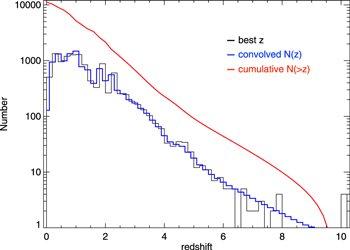
Figure 20. Redshift distribution of S/NFIR+mm > 5 sources. The black histogram shows the distribution of the best-fit redshifts from SED fitting. The uncertainty-convolved redshift distribution is shown as the blue histogram, while its cumulative distribution N(>z) is shown in red.
Download figure:
Standard image High-resolution image7.1. Candidate Selection at z > 4
There are three main classes of candidate z > 4 galaxies: (1) galaxies in our prior sample and with an existing optically based photometric redshift (as in L18, we eventually rederive a redshift from FIR SED fitting, constrained to be within 10% of the optical (1 + z) to avoid catastrophic failures); (2) galaxies in our prior sample for which no optical photometric redshift exists, mostly because they were selected from radio and lack an obvious match to the Ks-selected catalogs (we only have an FIR redshift here); and (3) additional sources added from the residual maps after the first-pass photometry (here also we only have an FIR redshift, and some of these are possibly spurious sources or unresolved blends; see also L18).
The FIR-based photometric redshifts from SED fitting are derived by considering the χ2 of the fit as a function of redshift and applying a Δχ2 = 2.5 criterion (corresponding to the 90% probability confidence) to determine the uncertainty of the redshift estimate following Avni (1976). High-z candidates are fitted using the Magdis et al. (2012) SB template for the dusty SF component, which in practice is GN20. This is appropriate regardless of the nature of SB or MS galaxies, given that even MSs have fairly warm SEDs at z > 4 (Béthermin et al. 2015; Schreiber et al. 2017). Still, the intrinsic SED shape as driven by dust temperature might have substantial variations among high-z galaxies. However, our approach is likely conservative, as GN20 at z = 4 has a relatively low dust temperature (Tdust = 35 K) compared to other z > 4 dusty star-forming galaxies (e.g., Smolčić et al. 2015; Riechers et al. 2017). If using some of the latter as templates, the redshifts would have been higher by up to 20%–25% (or about 5% × (1+z), depending on the template). We were also careful of using full AGN (Mullaney et al. 2011) and SF (Magdis et al. 2012) decomposition of the SED only in the presence of sufficient S/N in the photometry for allowing this, e.g., good detections in the mid-IR as well as FIR/(sub)mm ranges. When such a condition was lacking, we considered only the dusty SF component, to avoid cases in which the hot AGN SED would spuriously produce very high-redshift solutions with low by dominating the SED fit. Further details of the dust temperature–redshift degeneracies are discussed in Section 7.2.

Figure 21 (top panel) shows the distribution of redshift errors for the three classes. It is obvious that the redshift uncertainty can grow to be fairly large for objects where only the FIR SED is used to constrain it. As a result, we decided to limit the discussion of high-redshift candidates to those objects satisfying . Consequently, among significantly FIR-detected sources with existing , we obtain 31 sources with for class (1) above. Among 420 (mainly radio) sources lacking an optical photometric redshift, we select 20 sources with for class (2) above. There are 126 additional sources from the SCUBA2 residual image that reach (see Section 4.5), and 34 of them have and are in class (3). In total, we have 85 sources with as our final sample of high-redshift candidates. In the first three panels of Figure 23, we present examples that represent the different classes of candidates: (1) prior with , (2) radio prior without , and (3) additional source with IRAC counterpart.


Figure 21. Selection of high-redshift candidates and SFR–redshift diagram. Sources below the red dashed line (i.e., zphot,FIR − Δzphot,FIR > 4) are selected as our high-redshift candidates.
Download figure:
Standard image High-resolution imageNote that no additional candidates with are selected from the SPIRE residual image, which is typically at a lower redshift. The relative sensitivity of the SCUBA2 850 μm map is substantially higher than that of any SPIRE band for star-forming galaxies. Also, no further residual source candidates at are found from the AzTEC and MAMBO maps. These bands were fitted after the SCUBA2 residual sources were already added. They generally support the reality of the SCUBA2 residual sources.


7.2. Redshift–Dust Temperature Degeneracy
Using the far-IR colors of a galaxy to determine its redshift (in the absence of zspec) is known to suffer from the so-called Tdust−redshift degeneracy. In particular, the same colors could be fit by a colder template placed at lower redshift or by a warmer template placed at higher z. To quantify this degeneracy but also determine how the uncertainties in optical zphot affect the derivation of the dust temperature, or similarly of the mean radiation field, <U> = LIR/Mdust, we perform the following simulation. We build DL07 models (Draine & Li 2007) with representative γ, qPAH, Umin, and <U> parameters following Magdis et al. (2012) and calculate flux densities at the MIPS 24 μm, PACS, SPIRE, and SCUBA2 850 μm bands by placing the template at a wide range of fixed redshifts (zor = 0–6 with a step of 0.01). We then perform SED fitting using the full suite of DL07 models, fixing the redshift first at zmax = zor + Dz × (1 + zor) and then at zmin = zor −Dz ×(1 + zor), where Dz = 0.03, corresponding to the average photo-z uncertainty in the COSMOS field (Laigle et al. 2016). Thus, at each redshift, we derive three <U> values—, , and —and quantify the impact of the photo-z uncertainty in <U> by considering and . Our analysis yields an offset between the input and the extracted <U> with the case of zmin (zmax) systematically overestimating (underestimating) the true <U> by 15%. We conclude that the uncertainty in zphot,FIR introduces an extra small (at least for the case of Δz = 0.03 × (1 + z)) uncertainty of 15% in the determination of <U>. Repeating the process for the case of a modified blackbody (MBB) with a single Tdust and fixed β = 1.8 yields an uncertainty in the derived Tdust of ∼5%.


Furthermore, both MS and SB galaxies at any redshift are expected to exhibit a range of intrinsic <U> values (ΔU). Consequently, ΔU is expected to introduce an uncertainty in the far-IR-based zphot,FIR (Δzphot,FIR = zspec − zphot,FIR). In order to quantify Δzphot,FIR, we first need to adopt a reasonable value for ΔU. Since <U> ∝ LIR/Mdust ∝ LIR/(Mgas × Z) ∝SFE/Z (e.g., Magdis et al. 2012), where Z is the gas-phase metallicity, we can estimate the intrinsic range of <U> in terms of variations of star formation efficiency (SFE) and Z within and outside the MS. Assuming the various relations reported in the literature between SFE, distance from the main sequence (ΔMS), and Z (e.g., Magdis et al. 2012; Sargent et al. 2014; Tacconi et al. 2018), we estimate an intrinsic variation of ΔU ≈ 0.1–0.2 dex for MS galaxies. This is in agreement with the empirically determined 0.2 dex variation reported by Magdis et al. (2012) for local normal galaxies. Performing simulations as outlined above, we find that ΔU = 0.1–0.2 dex corresponds to Δzphot,FIR ≈ 0.06–0.1 × (1 + z). We note that a similar estimate is reached for SBs at any redshift, assuming a range in gas depletion timescale of 50–200 Myr. Thus, we conclude that the intrinsic variation of the shape of the far-IR SED of both MS and SB galaxies at any redshift introduces an intrinsic uncertainty of Δzphot,FIR ≈ 0.06–0.1 × (1 + z) that should be taken into account along with the uncertainties introduced by the photometric errors and the varying photometric coverage.
7.3. An Interesting Case of Possible Lensing
In some cases, the high-redshift candidates are interestingly coincident with previously existing low-redshift priors in our sample that were discarded for fitting at some longer wavelengths, but where a strong detection was later found in our procedure (often a residual source). This is similar to the case of source ID20003080 (AzTEC/C160) shown in Figure 22. This source is coincident with an early-type galaxy with known spectroscopic redshift that is associated with a mass-selected prior (ID659416), which is fitted at PACS bands while excluded at longer wavelengths because it is obviously too faint. Thanks to its radio detection, we already knew in this case of the presence of the very close (12 separation) radio source ID20003080 (i.e., Cosbo-7 in Bertoldi et al. 2007, AzTEC/C160 in Aretxaga et al. 2011) that is afterward solidly detected at SCUBA2 850 μm (S/N850 μm = 8.2) and MAMBO 1.2 mm (S/N1.2 mm = 7.4). Source ID20003080 appears to be a high-redshift galaxy that is aligned with (and perhaps gravitationally lensed by) an early-type galaxy at z = 0.36, likely part of a group or poor cluster of galaxies at the same redshift (see the RBG image in Figure 22, top right panel). We obtain a photometric redshift z = 4.0 ± 0.6 by fitting 24 μm to radio photometry.


Figure 22. Likely case of a gravitationally lensed dusty galaxy, ID20003080 (also known as Cosbo-7 in Bertoldi et al. 2007 and AzTEC/C160 in Aretxaga et al. 2011). We show the multiband cutouts centered on this source in the first panel and a color image (B, z, and Ks bands) in the second panel. The other panels show the SEDs of the z = 0.36 elliptical ID659416 and the lensed ID20003080.

Download figure:
Standard image High-resolution imageOther very similar cases, with background sources at possibly even higher redshift, are ID85004261 and ID20003117 (see Table 3 and Appendix D). Investigating their nature in detail is left to future work.
7.4. AGN Components at

We find 17 sources among our robust sample at that require an AGN component for their SED fitting (see Table 2). The criterion adopted to conclude this requires that the AGN flux normalization divided by its total uncertainty range () is larger than 2. This is supported by visual inspection and appears to be reliably returning reasonable results. In this AGN sample, there are eight sources with that we consider to be solid candidates, and the remaining nine sources with are considered to be tentative. The bolometric luminosities of the AGNs range over a quite remarkable erg s−1, fully in the QSO regime. We show their multiband cutouts and SEDs in Appendix D, where the AGN component is marked by the red curve in the SED panel.


Table 2. High-redshift Candidates that Fitted with a Significant AGN Component
| ID | zphot,opt | zspec | S/NFIR+mm | zphot,FIR | LIR,SF | Lbol,AGN |
|---|---|---|---|---|---|---|
| 223720 | 4.19 | ⋯ | 6.9 | 4.66 ± 0.28 | 5.5 ± 0.3 | 7.8 ± 2.4 |
| 339785 | 4.92 | ⋯ | 5.2 | 5.45 ± 0.45 | 5.3 ± 0.2 | 54.6 ± 17.3 |
| 347052 | 4.34 | ⋯ | 5.6 | 4.82 ± 0.14 | 3.8 ± 0.4 | 21.3 ± 7.9 |
| 551174 | 4.21 | ⋯ | 5.3 | 4.68 ± 0.16 | 6.1 ± 0.3 | 6.9 ± 2.7 |
| 556890 | 4.49 | 4.63 | 9.6 | 4.63 | 8.9 ± 0.1 | 16.1 ± 1.6 |
| 578482 | 4.32 | ⋯ | 10.7 | 4.75 ± 0.22 | 6.1 ± 0.4 | 8.8 ± 3.3 |
| 599184 | 4.41 | ⋯ | 7.6 | 4.89 ± 0.49 | 4.7 ± 0.4 | 8.5 ± 4.1 |
| 613818 | 4.47 | ⋯ | 6.8 | 4.67 ± 0.49 | 5.9 ± 0.8 | 12.5 ± 4.3 |
| 632541 | 4.29 | ⋯ | 6.5 | 4.77 ± 0.38 | 4.4 ± 0.5 | 12.0 ± 5.4 |
| 695002 | 4.31 | ⋯ | 13.7 | 4.79 ± 0.02 | 4.1 ± 0.2 | 48.8 ± 4.9 |
| 739920 | 4.42 | ⋯ | 7.7 | 4.76 ± 0.49 | 4.7 ± 0.3 | 13.6 ± 6.7 |
| 786213 | ⋯ | 4.34 | 32.6 | 4.34 | 15.3 ± 0.1 | 5.1 ± 0.7 |
| 965647 | 4.34 | ⋯ | 6.2 | 4.58 ± 0.19 | 4.5 ± 0.4 | 5.6 ± 2.7 |
| 10008348 | 4.16 | 4.45 | 5.2 | 4.45 | 5.6 ± 0.1 | 8.4 ± 1.2 |
| 10015010 | 3.91 | ⋯ | 8.4 | 4.35 ± 0.18 | 5.5 ± 0.3 | 11.0 ± 2.9 |
| 10137954 | ⋯ | 4.64 | 8.0 | 4.64 | 0.2 ± 0.2 | 34.9 ± 2.4 |
| 10213589 | 4.66 | ⋯ | 7.1 | 4.15 ± 0.03 | 4.2 ± 0.2 | 23.6 ± 4.9 |


Download table as: ASCIITypeset image
For the 85 z > 4 candidates, the sum of the SFR is . The bolometric AGN luminosity contained among AGN detections adds up to erg s−1, corresponding to an integrated black hole accretion rate of . The ratio of the black hole accretion rate to the SFR is thus 2 × 10⁻³, close but higher than the universal ratio discussed in Mullaney et al. (2012) despite the IR selection that should favor star formation. This might suggest some evolution toward stronger AGN activity in these sources that should be confirmed with further studies. The number density of the 17 objects in COSMOS (assuming volume within 4 < z < 5) is ϕ ∼ 8 × 10⁻⁷ Mpc−3 dex−1, which matches reasonably well with the X-ray luminosity function extrapolations from Vito et al. (2018), assuming a bolometric correction of Lbol = 25 × LX,2–10 keV. Our AGN detections are predicted to have X-ray fluxes of (2.9–31.1) × 10−15 erg cm−2 s−1 at 0.5–2 keV in the case of no obscuration, which would make them all detectable with the limiting depth of available X-ray imaging data (2.2 × 10⁻¹⁶ erg cm−2 s−1 at 0.5–2 keV) in the Chandra-COSMOS legacy survey (Civano et al. 2016). However, only two sources, ID10008348 and ID10137954, are cross-matched with the point-source catalog of Civano et al. (2016). These X-ray sources show very high obscuration with Lbol/LX,2–10 keV ∼ 300, even higher than the X-ray bolometric correction factors of Compton-thick AGNs in Brightman et al. (2017). The low X-ray detection rate and large Lbol/LX ratio clearly suggest that our IR-selected AGNs are heavily obscured in the X-ray, consistent with the current understanding of high-redshift populations (Vito et al. 2018).


7.5. Counterparts for Candidates Found in Residual Images
We list the 34 additional high-z candidates in Table 3. Given that the positions of these additional sources are blindly extracted from the SCUBA2 residual image that has a beam FWHM = 11'', we visually searched for counterparts in SPLASH, VLA 3 GHz, and ALMA 1.2 mm (M. Aravena et al. 2018, in preparation) images with a tolerance of 5'' and set the coordinates of their counterparts as their final positions. We find that 13 additional sources have a well-defined counterpart in the SPLASH and/or VLA and/or ALMA images. The counterparts are presented in cutouts in Appendix D and listed in Table 3. These associations are unlikely to happen by chance and appear robust: by cross-matching to the COSMOS2015 catalog for SPLASH and to our VLA catalog, we would expect only 0.03 chance coincidences per 5'' radius aperture, down to the flux limits reached in these probes. This suggests at most ∼1 spurious association among the 34 additional candidates. The identification of these 13 sources with counterparts and solid detections at multiple FIR/(sub)mm wavelengths suggests that the spurious fraction among the additional candidates is quite contained.
Table 3. High-redshift Candidates Found among Additional Sources from the SCUBA2 Residual Map
| ID | R.A. (J2000) | Decl. (J2000) | Counterparta | Nameb | Distancec | S/NFIR+mm | S/N850 μm | SFRd | ΔSFRd | zphot,FIRe | Δzphot,FIRe |
|---|---|---|---|---|---|---|---|---|---|---|---|
| 85000019 | 150.24172 | 1.60795 | SPLASH, 3 GHz | ⋯ | 32 |
6.8 | 3.3 | 1194 | 309 | 5.8 | 1.3 |
| 85000436 | 149.40348 | 1.73843 | 3 GHz | ⋯ | 19 |
5.7 | 4.2 | 981 | 205 | 5.4 | 0.9 |
| 85000496 | 149.49761 | 1.77057 | ⋯ | ⋯ | ⋯ | 5.3 | 4.3 | 702 | 324 | 6.0 | 1.8 |
| 85000552 | 150.04723 | 1.78372 | ⋯ | ⋯ | ⋯ | 5.5 | 3.3 | 534 | 104 | 5.5 | 1.4 |
| 85000762 | 149.53400 | 1.85461 | ⋯ | ⋯ | ⋯ | 6.4 | 3.8 | 528 | 131 | 4.8 | 0.8 |
| 85000922 | 150.49660 | 1.90440 | SPLASH | ⋯ | 22 |
6.2 | 3.8 | 1232 | 343 | 6.3 | 1.3 |
| 85001050 | 149.98028 | 1.93565 | ⋯ | ⋯ | ⋯ | 5.1 | 4.1 | 704 | 119 | 5.8 | 1.6 |
| 85001505 | 149.46728 | 2.09288 | SPLASH | ⋯ | 23 |
6.4 | 4.9 | 816 | 205 | 5.9 | 1.4 |
| 85001571 | 150.02743 | 2.11300 | SPLASH | ⋯ | 04 |
5.0 | 2.8 | 488 | 24 | 7.0 | 2.3 |
| 85001674 | 150.30121 | 2.14766 | SPLASH, 3 GHz | ⋯ | 16 |
6.1 | 4.2 | 836 | 128 | 5.1 | 0.9 |
| 85001756 | 149.87579 | 2.17826 | ⋯ | ⋯ | ⋯ | 5.8 | 4.1 | 621 | 151 | 7.2 | 2.2 |
| 85001929 | 150.10971 | 2.25753 | SPLASH | ⋯ | 08 |
12.9 | 6.8 | 692 | 151 | 5.2 | 0.5 |
| 85001969 | 149.97064 | 2.31366 | ALMA | AzTEC/C71 | 30 |
5.5 | 4.5 | 606 | 103 | 7.9 | 2.2 |
| 85002134 | 150.24795 | 2.38802 | ⋯ | ⋯ | ⋯ | 5.7 | 3.3 | 850 | 107 | 10.0 | 1.1 |
| 85002215 | 150.10063 | 2.33484 | SPLASH, 3 GHz | AzTEC/C114 | 35 |
9.6 | 6.7 | 721 | 47 | 5.9 | 0.8 |
| 85002966 | 149.42140 | 2.57688 | ⋯ | ⋯ | ⋯ | 7.6 | 5.2 | 692 | 112 | 4.7 | 0.7 |
| 85003151 | 150.02104 | 2.63323 | ⋯ | AzTEC/C132 | ⋯ | 5.5 | 3.3 | 678 | 154 | 6.2 | 1.7 |
| 85004261 | 150.05635 | 2.57327 | ALMA, 3 GHz | AzTEC/C10 | 26 |
8.3 | 5.8 | 1009 | 267 | 7.2 | 2.2 |
| 85005253 | 150.41618 | 1.90769 | ⋯ | ⋯ | ⋯ | 5.2 | 4.3 | 1413 | 223 | 8.6 | 1.7 |
| 85005277 | 150.57793 | 1.93306 | ⋯ | ⋯ | ⋯ | 5.0 | 3.3 | 1425 | 316 | 10.0 | 2.3 |
| 85005285 | 150.68263 | 1.95067 | 3 GHz | ⋯ | 49 |
5.1 | 3.1 | 1053 | 509 | 7.6 | 2.2 |
| 85005338 | 149.96455 | 1.98236 | ⋯ | ⋯ | ⋯ | 5.2 | 3.3 | 898 | 144 | 10.0 | 1.9 |
| 85005422 | 149.98861 | 2.09413 | ⋯ | ⋯ | ⋯ | 5.1 | 3.4 | 601 | 57 | 7.8 | 2.1 |
| 85005464 | 149.68279 | 2.09387 | ⋯ | ⋯ | ⋯ | 5.5 | 2.7 | 570 | 152 | 5.4 | 1.4 |
| 85005517 | 150.64576 | 2.14272 | ⋯ | ⋯ | ⋯ | 5.0 | 2.5 | 934 | 272 | 6.7 | 1.8 |
| 85005620 | 150.70247 | 2.25888 | ⋯ | ⋯ | ⋯ | 5.1 | 2.6 | 989 | 312 | 7.1 | 2.0 |
| 85005670 | 150.60669 | 2.31664 | ⋯ | ⋯ | ⋯ | 5.3 | 2.9 | 828 | 136 | 5.7 | 1.4 |
| 85005722 | 150.61282 | 2.41777 | ⋯ | ⋯ | ⋯ | 5.1 | 2.9 | 1171 | 267 | 5.6 | 1.5 |
| 85005759 | 149.78323 | 2.40500. | ⋯ | ⋯ | ⋯ | 5.1 | 3.2 | 504. | 93 | 5.9 | 1.8 |
| 85005769 | 150.36338 | 2.41572 | ⋯ | ⋯ | ⋯ | 5.9 | 3.2 | 993 | 287 | 5.3 | 1.1 |
| 85005926 | 149.95379 | 2.56544 | SPLASH, 3 GHz | ⋯ | 20 |
7.0 | 2.6 | 656 | 114 | 5.5 | 1.0 |
| 85005933 | 149.75172 | 2.58143 | ⋯ | ⋯ | ⋯ | 5.2 | 2.7 | 582 | 168 | 7.2 | 2.5 |
| 85005963 | 150.69766 | 2.60405 | ⋯ | ⋯ | ⋯ | 7.5 | 2.7 | 1176 | 574 | 6.0 | 1.6 |
| 85006141 | 150.45836 | 2.81048 | 3 GHz | ⋯ | 18 |
8.3 | 2.5 | 1199 | 473 | 6.0 | 1.4 |
Notes. We report here the result for our search of Spitzer IRAC and radio counterparts.
aCounterpart image. SPLASH: P. Capak; 3 GHz: Smolčić et al. (2017); ALMA: 1.2 mm continuum image (M. Aravena et al. 2018, in preparation). bReference name of the counterpart (Aretxaga et al. 2011). cDistance of additional source to its counterpart. dSFR and ΔSFR: median fit and uncertainty of SFR based on FIR+(sub)mm SED fitting, Chabrier IMF (Chabrier 2003). ezphot,FIR and Δzphot,FIR: the photometric redshift and uncertainty based on FIR+(sub)mm SED fitting.Download table as: ASCIITypeset image
Like for the other candidates, we fit their photometry at 100–1200 μm and 3 GHz using the GN20 template and an evolving qIR without an AGN component. The 3 GHz photometry is taken from counterparts in the VLA 3 GHz image, while for candidates without any counterpart, we do not fit the 3 GHz photometry. Note that there are three additional sources that result in a best-fit z = 10, the highest value that we allow. These three sources are only detected at (sub)mm wavelengths while their SEDs are weakly constrained by Herschel. Given the redshift errors Δzphot,FIR = 1.1–2.3, it is quite plausible that these sources are at more reasonable, lower redshifts. On the other hand, we notice that no counterpart is found for these sources, so they might also possibly be spurious detections in the SCUBA2 residual image, in some cases.
7.6. General Sample and Final Considerations on Redshift Estimates
The cosmic volume sampled by COSMOS, adopting a generous redshift range 4 < z < 8, is 7 × 10⁷ Mpc3, and the SFRD from our population in this volume is about . This seems quite low with respect to the total SFRD at these redshifts (Madau & Dickinson 2014; L18), as expected due to the shallower depths reached. We are likely still sampling the high-end tail of the luminosity function, albeit now with pretty fair statistics.

Ivison et al. (2016) selected a sample of 109 dusty star-forming galaxies with Herschel colors (S500 um ≥ 30 mJy, i.e., S500 um/S250 um ≥ 1.5 and S500 um/S250 um ≥ 0.85) in a 600 deg2 survey, estimated 32% of that sample to have z =4–6, and reported a number density of Mpc−3. The sources of Ivison et al. (2016) have a median infrared luminosity (LIR) ∼ 1.3 × 10¹³ L⊙, while our z > 4 sample reaches to fainter levels with a median LIR ∼ 8.0 × 10¹² L⊙ and down to LIR ∼ 3.6 × 10¹² L⊙. We detected 64 dusty star-forming galaxies at z = 4–6 (σ500 μm ∼ 3 mJy), implying a much higher space density than that in Ivison et al. (2016). Given that the completeness of our z > 4 sample is not yet constrained, detailed values for the space densities will be reported in a future paper.

Among the 85 candidates, there are six sources with confirmed spectroscopic redshift z > 4. Four of them are listed in Table 2, as they are fitted with an AGN component, while five of them are shown in Appendix D with their actual "zspec" marked in the SED panels. The last source with spectroscopic redshift is the source ID20007898 (i.e., AzTEC/C1 in Smolčić et al. 2012), as shown in the fourth panel of Figure 23, whose spectroscopic redshift zspec = 4.7 has been reported by Brisbin et al. (2017). As a test, we ignored the redshift of ID20007898 and fit its SED over z = 0–10 to derive a photometric zphot,FIR = 4.8 ± 0.25. This agrees well with the zspec, suggesting that our SED procedure is reasonable for giving photometric redshifts on z > 4 dusty galaxies. We have run the same test on IR-detected sources with zspec > 3 and shown the redshift comparison in Figure 24. Our IR SED-driven photometric redshift is in good agreement with the spectroscopic redshift for galaxies with significant FIR/(sub)mm detections, while it is perhaps somewhat underestimated in the case of galaxies with important AGN torus emission. The relevance of this hint is limited, of course, by low-number statistics. We find that in order to obtain a fair comparison between photometric and spectroscopic redshifts, the redshift uncertainties must be increased by adding in quadrature an extra component of about 10% of (1+z). This is of order of the systematic effect expected from dust temperature variations, as discussed in Section 7.2. The redshift errors associated with our sources currently only reflect the accuracy of their SEDs and do not include such systematic uncertainties. Once weighted by the (total) redshift uncertainties, the comparison in Figure 24 suggests that our FIR photometric redshifts are underestimated by 6% × (1 + z) (Δz ∼ 0.4), on average, confirming the idea that the FIR SED of GN20 is somewhat colder than the high-z average. Larger samples are required to bring these results to firmer footing.

Figure 23. Four examples of z > 4 candidates. We show the multiband cutouts on the left accompanying SED on the right. The instrument used, wavelength (in units of μm), and FoV are shown in green text in each cutout. The SEDs are fitted with a starburst-like template (green curve; Magdis et al. 2012) and a stellar component (blue curve; Bruzual & Charlot 2003).
Download figure:
Standard image High-resolution image
Figure 24. Comparison of photometric redshift and spectroscopic redshift of z > 3 sources. The size of the symbol is scaled by S/NFIR+mm. The red data points show sources fitted with an AGN component.
Download figure:
Standard image High-resolution imageThe multiband cutouts and SEDs of all candidates are presented in Appendix D. Redshift confirmation of as many as possible of these candidates is clearly needed, and we are planning observations with NOEMA, ALMA, and hopefully JWST in the future. Such further studies of these high-z candidates will be needed to finally validate their selection and understand critical issues like completeness, spurious fraction, actual redshift distribution (hence number densities), and others. Our photometric catalog in COSMOS will be the basis for such explorations.
8. Summary
In this work, we obtain (and publicly release) detailed "super-deblended" photometry for FIR-to-(sub-)millimeter imaging data sets in the COSMOS full 2 deg2 field, with the most accurate photometry information lying where complete prior information is available, i.e., in the 1.7 deg2 UltraVISTA area. In order to overcome the heavy blending problems introduced by the large beam size at the Herschel SPIRE and (sub)mm bands, we adopted the "super-deblending" technique that has been pioneered in the GOODS-North field by L18 and critically adapted it to the COSMOS field, where data at PACS, Spitzer/MIPS, and radio are shallower than in the GOODS-N field.
We selected a highly complete set of 194,428 priors for deblending the FIR-to-mm images. This prior catalog contains 88,008 detections from MIPS 24 μm and radio fitting and ∼1 × 10⁵ mass-selected priors from UltraVISTA catalogs.
In the deblending of the FIR/(sub)mm images, we improved the faint-source subtraction by only subtracting fluxes of galaxies with a reliable determination as predicted by the SED fitting. We calibrated and removed biases from this subtraction step using Monte Carlo simulations. This returned flux uncertainties with well-behaved Gaussian-like statistics.
A total of 11,220 galaxies are individually detected with a combined S/N > 5 over the FIR/(sub)mm wavelengths, including 770 detections at z ≥ 3 (mostly photometric). Comparing with photometric catalogs in the literature, the "super-deblended" photometry shows good agreement for bright sources and generally improved deblending at the faint end.
Quite notably, the "super-deblended" 850 μm photometry agrees remarkably well with ALMA archival data photometry, with a scatter that is consistent with the "super-deblended" photometric error, demonstrating that the "super-deblended" photometry is correctly derived and errors are statistically well defined.
Finally, we conservatively selected 85 robust high-redshift candidates with solid detections at FIR/(sub)mm wavelengths requiring z > 4 (we use z−zerror > 4). These candidates have often well-determined counterparts in IRAC and/or radio images and weak or no detection at the Ks band. Their SEDs suggest redshifts over z ∼ 4–7, including possibly some of the most distant galaxies known. Confirmation of redshifts by future observations is needed. This unique sample will allow us to statistically investigate the first generation of vigorous star formation in the early universe.
We are grateful to the full COSMOS team for their contributions in the buildup of such a rich multiwavelength data set. We thank the referee for useful comments and suggestions that helped improve the paper. We thank B. Magnelli, P. Lang, and the rest of the A3COSMOS team for providing the ALMA photometry for comparison. SJ acknowledges funding from the China Scholarship Council. SJ and QG acknowledge support from the National Key Research and Development Program of China (No. 2017YFA0402703) and the National Natural Science Foundation of China (No. 11733002). D.L. and Y.G. acknowledge support from the National Key Research and Development Program (No. 2017YFA0402704) and the National Natural Science Foundation of China (No. 11420101002). V.S., J.D., and I.D. acknowledge support from the European Union's Seventh Framework program under grant agreement 337595 (ERC Starting Grant, "CoSMass"). ES and DL acknowledge funding from the European Research Council (ERC) under the European Union's Horizon 2020 research and innovation program (grant agreement No. 694343). The National Radio Astronomy Observatory is a facility of the National Science Foundation, operated under cooperative agreement by Associated Universities, Inc. ALMA is a partnership of the ESO (representing its member states), NSF (USA), and NINS (Japan), together with the NRC (Canada), MOST and ASIAA (Taiwan), and KASI (Republic of Korea), in cooperation with the Republic of Chile. The Joint ALMA Observatory is operated by the ESO, AUI/NRAO, and NAOJ.
Appendix A: MIPS 24 μm Calibration Factor
We use a sample of significant IR detections at redshift 0.4 < z < 0.58, a redshift range where starburst and main-sequence galaxies have identical ratios of 24 μm fluxes to bolometric FIR fluxes, based on the Magdis et al. (2012) templates. In Figure 25, we compare the total SFR from the FIR SED fitting in our work with the SFR estimated only from the 24 μm flux on the basis of templates from Magdis et al. (2012). We only show sources with reliable detections, S/N24 μm > 5 and S/NFIR+mm > 5, and from both the COSMOS (this work) and GOODS-N (L18) fields. We find that in the COSMOS field, SFRs directly obtained from the FIR photometry (100 μm–1.2 mm) are higher than the 24 μm extrapolated ones by a factor of about 1.7, while this issue is not seen in the GOODS-N "super-deblended" catalog. The agreement in the GOODS-N field is, of course, by construction, given that the GOODS-N (and GOODS-S) data were used to construct the Magdis et al. (2012) templates, including the photometry at the mid-IR bands from Spitzer MIPS and IRS.

Figure 25. The SFR from FIR+mm SED fitting vs. SFR from 24 μm extrapolation (Magdis et al. 2012). All sources have redshift z = 0.4–0.58 with S/N24 μm > 5 and S/NFIR+mm > 5. Blue circles show sources in the GOODS-N field, while orange circles show sources in the COSMOS field. The identity line is shown in red, while the median linear fit of the COSMOS sources is shown in green (i.e., 1.7× the identity line).
Download figure:
Standard image High-resolution imageWe have also checked that this effect remains if we are using the SFRs only based on 100 and 160 μm fluxes in the "super-deblended" catalog, which are subjected to much less blending than, e.g., SPIRE bands.
A similar effect is also reported by Ilbert et al. (2015; see their Figure 1), where they found evidence for the need for a factor of 1.5 upscaling of 24 μm fluxes in COSMOS when using the template of Magdis et al. (2012), although this is reduced to a factor of 1.2 with Dale & Helou (2002) templates. They suggested that this difference might be due to the use of different data reduction pipelines, as well as the combined uncertainties in the absolute calibration of MIPS and Herschel data.
Overall, it is difficult to conclude if this is really a problem of the COSMOS photometry, as it might instead be a problem with the GOODS photometry, or a mix thereof. Also, it might apply at least in part to the overall PACS and SPIRE photometry in COSMOS versus GOODS. What appears to be more reliable is that the interpretation of COSMOS 24 μm to FIR SEDs with Magdis et al. (2012) templates (or, more in general, their comparison to GOODS-N fluxes) requires some rescaling. A possible solution to make the comparison consistent is the multiplication of COSMOS 24 μm fluxes by a factor of 1.5–1.7, which is the range where our current analysis and that of Ilbert et al. are converging.
Appendix B: Photometry Image Products
We present the photometry image products at each band here. All images have the same scaling and share the color bar in terms of S/N, following Figure 9 (see also the caption there). Figure 26 shows image products in the MIPS 24 μm, VLA 3 and 1.4 GHz, and PACS 100 μm images, where no faint source is subtracted from their original images. Figures 27 and 28 show image products in 160 um to 1.2 mm images.
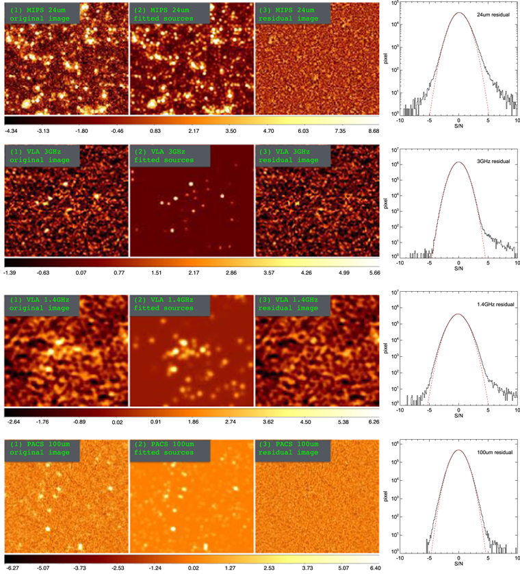
Figure 26. Photometry image products at MIPS 24 μm, VLA 3 and 1.4 GHz, and PACS 100 μm. Panel (1) is a portion of the original map of each band. Panel (2) shows the galfit best-fitting model image of fitted priors, and panel (3) is the residual image of panels (1) and (2). Image values and histograms are expressed in terms of S/N (see also the caption of Figure 9).
Download figure:
Standard image High-resolution image
Figure 27. Photometry image products at PACS 160 μm and SPIRE 250, 350, and 500 μm. See descriptions in text.
Download figure:
Standard image High-resolution image
Figure 28. Photometry image products at SCUBA2 850 μm, AzTEC 1.1 mm, and MAMBO 1.2 mm. See descriptions in text.
Download figure:
Standard image High-resolution imageAppendix C: Simulation Correction Analyses
Analog to Appendix B in L18, we present here the figures of our simulation-based correction recipes at each band. For example, in Figure 29, the simulation data points are binned by four measurable parameters: the galfit flux uncertainty normalized by the local rms noise at the source position (σgalfit/σrmsnoise; first column); the residual flux within one PSF beam area in the residual image, also normalized by the local rms noise (Sresidual/σrmsnoise; the second column); the crowdedness parameter (third column); and the normalized subtraction Ssubtracted/σrmsnoise (fourth column). Bins are indicated by the dashed vertical lines in the first and second rows.

Figure 29.
Simulation correction analyses at SPIRE 250 μm. See descriptions in text. (The complete figure set (11 images) is available.)
Download figure:
Standard image High-resolution image
Figure 30.
Multiband cutouts and SEDs of high-redshift candidates. (The complete figure set (85 images) is available.)
Download figure:
Standard image High-resolution imageFrom left to right, the panels are in the same four-parameter order. The first row shows the difference between the input and output flux of each simulated source (Sin − Sout; i.e., the flux bias) versus the four parameters, which is fitted by a third-order polynomial function (red curve). The second row shows the flux difference divided by the flux uncertainty (Sin − Sout)/σ) versus the four parameters. The scatter in each bin is considered as the correction factor that needs to be applied to σ. Uncorrected and corrected data are shown in blue and red, respectively. After correction, the scatter of (Sin − Sout)/σ in each bin is very close to 1.0, indicating that the corrected σ is statistically consistent with the scatter of Sin − Sout. We fit a third-order polynomial function to the bin-averaged flux uncertainty correction factor on each parameter, which is shown as the red curve. The right axis indicates its value. The third row shows the histogram of (Sin − Sout)/σ before and after correction of each parameter. Its shape after correction (i.e., the red histogram) becomes a well-behaved Gaussian distribution (i.e., symmetric and has a Gaussian width of 1.0) and is much better than the uncorrected one (i.e., the blue histogram). The fourth row shows the histogram of the flux. The fifth row shows the histogram of the flux uncertainty.
Appendix D: High-redshift Candidates
We present cutouts and SEDs of high-redshift candidates here. As two candidates shown in Figures 30, we show cutouts of the UltraVISTA Ks, SPLASH 3.6 and 4.5 μm, VLA 3 GHz, MIPS 24 μm, Herschel, SCUBA2, and MAMBO images on the left and the accompanying SED on the right. The instrument, wavelength (in units of μm), and FoV are shown in green text in each cutout. The scheme of the symbols in the SED panels is identical to that in Figure 7.
Table 4. COSMOS "Super-deblended" Photometry Catalog
| Name | Units | Description |
|---|---|---|
| ID | ⋯ | Identifier |
| R.A. | deg | Right ascension |
| Decl. | deg | Declination |
| zphot | ⋯ | Photometric redshift from optical/near-infrared catalogs |
| zspec | ⋯ | Spectroscopic redshift |
| zspec_ref | ⋯ | Reference code of spectroscopic redshift |
| Mstar | M⊙ | Stellar mass in Chabrier IMF |
| SNR_IR | ⋯ | Super-deblended 100 μm–to–1.2 mm combined S/N |
| goodArea | ⋯ | Super-deblended "goodArea" flag |
| z_IR | ⋯ | Super-deblended IR-to-radio photometric redshift |
| ez_IR | ⋯ | Super-deblended IR-to-radio photometric redshift error |
| SFR_IR | M⊙ yr−1 | Super-deblended SED fit SFR |
| eSFR_IR | M⊙ yr−1 | Super-deblended SED fit SFR error |
| Kmag | ⋯ | Ks-band magnitude |
| Fch1 | mJy | Spitzer IRAC 3.6 μm flux |
| dFch1 | mJy | Spitzer IRAC 3.6 μm flux error |
| Fch2 | mJy | Spitzer IRAC 4.5 μm flux |
| dFch2 | mJy | Spitzer IRAC 4.5 μm flux error |
| Fch3 | mJy | Spitzer IRAC 5.8 μm flux |
| dFch3 | mJy | Spitzer IRAC 5.8 μm flux error |
| Fch4 | mJy | Spitzer IRAC 8.0 μm flux |
| dFch4 | mJy | Spitzer IRAC 8.0 μm flux error |
| F24 | mJy | Super-deblended Spitzer MIPS/24 μm flux |
| dF24 | mJy | Error in F24 |
| F100 | mJy | Super-deblended Herschel/PACS 100 μm flux |
| dF100 | mJy | Error in F100 |
| F160 | mJy | Super-deblended Herschel/PACS 160 μm flux |
| dF160 | mJy | Error in F160 |
| F250 | mJy | Super-deblended Herschel/SPIRE 250 μm flux |
| dF250 | mJy | Error in F250 |
| F350 | mJy | Super-deblended Herschel/SPIRE 350 μm flux |
| dF350 | mJy | Error in F350 |
| F500 | mJy | Super-deblended Herschel/SPIRE 500 μm flux |
| dF500 | mJy | Error in F500 |
| F850 | mJy | Super-deblended JCMT/SCUBA2 850 μm flux |
| dF850 | mJy | Error in F850 |
| F1100 | mJy | Super-deblended ASTE/AzTEC 1.1 mm flux |
| dF1100 | mJy | Error in F1100 |
| F1200 | mJy | Super-deblended IRAM/MAMBO 1.2 mm flux |
| dF1200 | mJy | Error in F1200 |
| F10cm | mJy | Super-deblended VLA 3 GHz flux |
| dF10cm | mJy | Error in F10cm |
| Smolcic | ⋯ | Flag of whether the original 3 GHz photometry is from Smolčić et al. (2017) |
| F10cm_1arc5 | mJy | Super-deblended VLA 3 GHz flux in 15 convolved image |
| dF10cm_1arc5 | mJy | Error in F10cm_1arc5 |
| F10cm_2arc | mJy | Super-deblended VLA 3 GHz flux in 2'' convolved image |
| dF10cm_2arc | mJy | Error in F10cm_2arc |
| xfAGN | Super-deblended SED best-fit AGN luminosity | |
| xeAGN | Error in xfAGN | |
| xfTOT | Super-deblended SED fit total luminosity | |
| xeTOT | Error in xfTOT | |
| xf70 | mJy | Super-deblended SED predicted flux density at 70 μm |
| xe70 | mJy | Error in xf70 |
| xf100 | mJy | Super-deblended SED predicted flux density at 100 μm |
| xe100 | mJy | Error in xf100 |
| xf160 | mJy | Super-deblended SED predicted flux density at 160 μm |
| xe160 | mJy | Error in xf160 |
| xf250 | mJy | Super-deblended SED predicted flux density at 250 μm |
| xe250 | mJy | Error in xf250 |
| xf350 | mJy | Super-deblended SED predicted flux density at 350 μm |
| xe350 | mJy | Error in xf350 |
| xf500 | mJy | Super-deblended SED predicted flux density at 500 μm |
| xe500 | mJy | Error in xf500 |
| xf850 | mJy | Super-deblended SED predicted flux density at 850 μm |
| xe850 | mJy | Error in xf850 |
| xf1100 | mJy | Super-deblended SED predicted flux density at 1100 μm |
| xe1100 | mJy | Error in xf1100 |
| xf1200 | mJy | Super-deblended SED predicted flux density at 1200 μm |
| xe1200 | mJy | Error in xf1200 |
| xf2000 | mJy | Super-deblended SED predicted flux density at 2000 μm |
| xe2000 | mJy | Error in xf2000 |
| xf3000 | mJy | Super-deblended SED predicted flux density at 3000 μm |
| xe3000 | mJy | Error in xf3000 |
| xf10cm | mJy | Super-deblended SED predicted flux density at 10 cm |
| xe10cm | mJy | Error in xf10cm |
| xf20cm | mJy | Super-deblended SED predicted flux density at 20 cm |
| xe20cm | mJy | Error in xf20cm |
| Ubest | ⋯ | Mean interstellar radiation field strength of SED best-fit dust template |
| Chi2_min | ⋯ | Super-deblended SED χ2 of fitted data points |
| S_chi2_min | ⋯ | Super-deblended SED χ2 of fitted data points for stellar component of the SED |
| R_chi2_min | ⋯ | Super-deblended SED χ2 of fitted data points for dust component of the SED |
| Type_FIR | ⋯ | Super-deblended SED fitting's Type_FIR flag |
| Type_SED | ⋯ | Super-deblended SED fitting's Type_SED flag |
| Type_AGN | ⋯ | Super-deblended SED fitting's Type_AGN flag |


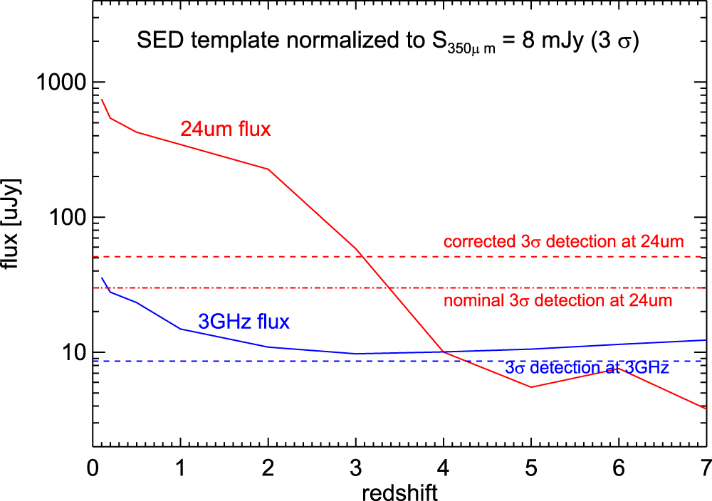
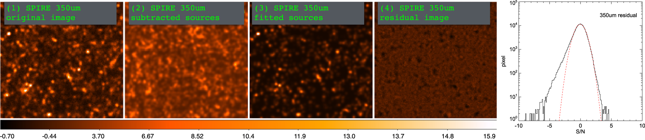
Notes. This table is available in its entirety in FITS format in the .tar.gz package. A portion is shown here for guidance regarding its form and content.
Footnotes
- 15
The completeness of the prior sample for galaxies that have intrinsic flux above some detectable threshold (e.g., >3σ) in an image under exam is defined as the fraction of them for which a prior is actually present in the prior sample.
- 16
As discussed later, we find evidence that the 24 μm photometry in COSMOS should be scaled up by a factor of 1.5–1.7 in order to be consistent with the GOODS 24 μm to FIR flux ratios. This would imply that the actual rms sensitivity is ∼15–17 μJy at this band and ∼3× shallower than GOODS-N.
- 17
The situation might change in the future from completion of the Spitzer Large Area Survey with Hyper-Suprime-Cam photometry (SPLASH; PI: P. Capak).
- 18
We only use publicly available redshifts for this work, taken from Colless et al. (2001; 2dF); Prescott et al. (2006; MMT); Skrutskie et al. (2006; 2MASS); Lilly et al. (2007, 2009; zCOSMOS); Trump et al. (2007; IMACS); Kartaltepe et al. (2010); Coil et al. (2011; PRIMUS); Faure et al. (2011); Fu et al. (2011); Roseboom et al. (2012); Onodera et al. (2012, 2015; MOIRCS), Balogh et al. (2014; GEMINI-S); Comparat et al. (2015; FORS2); Silverman et al. (2015; FMOS); Perna et al. (2015; SINFONI); Yun et al. (2015); Kriek et al. (2015; MOSDEF); Marchesi et al. (2016); Momcheva et al. (2016; 3D-HST); Nanayakkara et al. (2016; ZFIRE); van der Wel et al. (2016; LEGA-C); Masters et al. (2017; DEIMOS-C3R2); Tasca et al. 2017; VUDS); Marsan et al. (2017; NIRSPEC); Abolfathi et al. (2018; SDSS DR14) and Hasinger et al. (2018; DEIMOS).
- 19
A Gaussian PSF is a very good approximation of the true beam, especially given the fact that the large number of VLA antennas does not result in significant sidelobes and that a Gaussian PSF is used for reconstruction during the CLEAN process (Schinnerer et al. 2010; Smolčić et al. 2017). On the other hand, the comparison of our measurements to the catalogs confirms this.
- 20
For these 8200 XID+ 24 μm–detected priors missing from our work, we tend to believe they come from mismatches between our accurate positions from our Ks and radio catalogs and the blind-extracted 24 μm sources in XID+.
- 21
- 22