
Abstract
Gas bubbles submerged in a dielectric liquid and driven by an electric field can undergo dramatic changes in both shape and volume. In certain cases, this deformation can enhance the distribution of the applied field inside the bubble as well as decrease the internal gas pressure. Both effects will tend to facilitate plasma formation in the gas volume. A practical realization of these two effects could have a broad impact on the viability of liquid plasma technologies, which tend to suffer from high voltage requirements. In this experiment, bubbles of diameter 0.4–0.7 mm are suspended in the node of a 26.4 kHz underwater acoustic standing wave and excited into nonlinear shape oscillations using ac electric fields with amplitudes of 5–15 kV cm−1. Oscillations of the deformed bubble are photographed with a high-speed camera operating at 5130 frames s−1 and the resulting images are decomposed into their axisymmetric spherical harmonic modes,
 , using an edge detection algorithm. Overall, the bubble motion is dominated by the first three even modes l = 0, 2 and 4. Electrostatic simulations of the deformed bubble's internal electric field indicate that the applied field is enhanced by as much as a factor of 2.3 above the nominal applied field. Further simulation of both the pure l = 2 and l = 4 modes predicts that with additional deformation, the field enhancement factors could reach as much as 10–50.
Export citation and abstract BibTeX RIS
1. Introduction
Electrical discharges occurring in water produce a variety of chemically reactive products [1–3], which have garnered considerable interest for potential applications ranging from the decomposition of volatile organic compounds in industrial waste to the development of point-of-use water purification [4–6]. The ignition of plasma directly within these environments, however, is limited by the large breakdown strength of liquids, which at ∼1 MV cm−1, imposes impractical voltage and energy requirements on the design of real devices [7]. This difficulty can be alleviated by producing plasma in a secondary gas discharge and then injecting it into the liquid [8]. There are a variety of techniques investigated for this purpose, including surface discharges [9], pulsed corona discharges [10], glow discharge electrolysis [11, 12], dielectric barrier discharges [13] and gliding arc discharges [14, 15]. These approaches share among them the limitation that reactive products must be produced at the liquid surface, thereby limiting their penetration into the liquid and consequently their capacity to process large throughputs. One way to circumvent this difficulty is by producing plasma inside gas bubbles that are distributed throughout the water [16–18]. This technique maintains the low breakdown environment of the gas while increasing the penetration of reactivity into the liquid volume. Furthermore, a sufficiently dense cluster of such bubbles can stimulate the 'hopping' of streamer discharges from bubble to bubble [19]. Another advantage of this approach derives from the permittivity change that typically occurs across the bubble-liquid boundary. A large change in permittivity can distort or 'focus' the applied electric field, often resulting in amplification within the bubble volume. In the case of a uniform field applied to an air bubble in water, the internal field is increased by a factor of nearly 3/2 [20]. In general, field enhancement is sensitive to the shape of the bubble and can be very large in cases where the curvature of the surface is extreme [21].
Despite these apparent advantages, the ignition of plasma in isolated bubbles, to the author's knowledge, has yet to be demonstrated experimentally. This is most likely due to the difficulty in transmitting a large electric field across a high permittivity liquid and into the gas bubble. The electric field enhancement resulting from extreme bubble shape distortions, as described above, can be used as a tool to overcome this problem and facilitate plasma production inside submerged bubbles. If the bubble is deformed to a shape strategically designed to enhance the field, then plasma ignition within the bubble gas could be achieved at reduced voltages, and at potentially lower energy cost. In this paper, we explore the use of this shape effect by distorting a single bubble and estimating the change to its internal electric field. In this case, the distorting force is provided by an ac electric field, which act on the dielectric fluid surrounding the bubble. One advantage of this approach is that the driving electric field can also be used to initiate breakdown within the bubble [22]. In addition, precise control of the shape, frequency and magnitude of the electric field are all simple for timescales associated with bubble oscillations (kHz for mm sized bubbles).
The electric stress acting on a homogeneous dielectric is determined by the Maxwell stress tensor [23],

Inside the body of a liquid, the force per unit volume is given by the divergence of
 . At the liquid surface, the normal stress is given by,

Here n is the unit vector normal to the surface. In the case of a gas bubble, the electric stress distorts the liquid boundary when it becomes comparable to the inward restorative force of the bubble's surface tension. The ratio of these two pressures is defined as the electrical Weber number [24],

Here R0 is the radius of the bubble and σ is the surface tension constant. For reference, an electric field of 4.5 kV cm−1 acting on a 1.0 mm diameter bubble (in water) will yield a Weber number equal to one. Under a sufficiently strong driving force the bubble's volume may increase. As the volume increases, the gas pressure decreases, resulting in a pressure difference between the ambient liquid and the bubble gas. This pressure gradient drives the diffusion of dissolved air from the liquid into the bubble in an attempt to reestablish equilibrium. If the bubble expansion is rapid enough, the gas pressure will temporarily be below atmosphere and will reduce the electric field required for breakdown [25]. This volume effect, serves as an additional mechanism to facilitate plasma formation within the bubble.
The dynamics of an air bubble driven by a time-varying electric field can be viewed as a superposition of discrete spherical harmonics modes [26]. In the case of axisymmetric motion, these reduce to the Legendre polynomials.
In (4), μ represents cos (θ) where θ is the polar angle in spherical coordinates. The coefficients, bl(t) can be solved by integrating against the corresponding Legendre polynomial,
In the case of unforced, linear motion (bl ≪ 1), the spherical harmonic components, Pl(μ ), oscillate at a characteristic frequency determined by the integer l [26]. The lowest coefficient, b0 is often referred to as the 'volume' mode because it represents an oscillation of the radius (and hence volume) while maintaining a spherical shape. This occurs at a characteristic frequency f0 given by,
Here p0 and ρ are the pressure and density of the surrounding liquid while k is the heat capacity ratio of the gas in the bubble. The remaining modes (l ⩾ 2) represent volume preserving perturbations of the Legendre polynomial pl(μ ), each with a characteristic frequency given by [26],

In the case of l = 1, P1 (θ) = μ, which is a simple translation along the z-axis. If the bubble has no net drift, then b1 is zero. To summarize, the 'volume' mode represents a shape preserving oscillation of the volume, while the various 'shape' modes represent volume preserving oscillations of the shape. The general motion is a superposition of these modes. Figure 1 shows the first two even shape modes, l = 2 and l = 4 for reference.
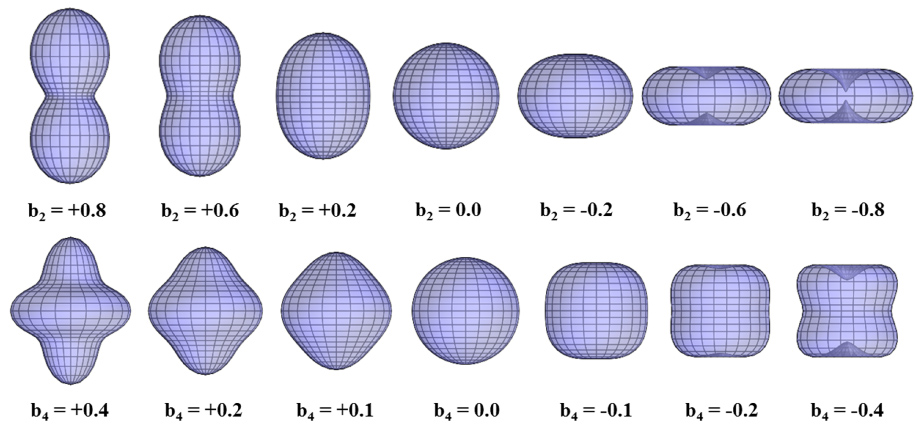
Figure 1. Spherical harmonic perturbations of the unit sphere for the l = 2 mode (top row) and the l = 4 mode (bottom row).
Download figure:
Standard imageThe spherical harmonics provide a convenient framework to describe distortions induced by an electric field. The approach taken in this work is to excite these modes individually by tuning the ac electric field to the frequencies given by (6) and (7). The resulting 'resonant' oscillations and subsequent distortion to the bubble's shape or volume will provide an experimental framework with which to examine the shape effect and volume effect.
To provide clarity into the relationship between the applied electrical stress and the resulting mode structure, consider an air bubble suspended in a liquid with permittivity ε and a uniform electric field
 . The electric stress acting normal to the unperturbed bubble surface can be calculated using (2) and is given by [20],

The pressure is highest at the equatorial plane (θ = π/2) where it squeezes the surface inwards. If the volume of the bubble is conserved, then the inward compression will force the bubble to stretch vertically, resulting in a shape closely resembling the l = 2 mode (see figure 1). Moreover, it has been determined experimentally that in the linear regime, a uniform field will excite only the l = 0 and l = 2 modes [27]. As discussed in the following section, the electric field profile used in this work is approximately uniform so it is expected that the l = 2 mode will play an important role in any observed bubble oscillations.
2. Experimental setup and methodology
2.1. Acoustic levitation
A controlled investigation of underwater bubbles can be accomplished by trapping them individually in an ultrasonic acoustic standing wave. Acoustic levitation of bubbles has been used extensively in prior investigations of bubble dynamics [28, 29] and sonoluminesence [30, 31]. The device used in this experiment, shown in figure 2, consists of a rectangular cell with 6.35 mm thick Plexiglas walls. A piezoelectric transducer was fed through the bottom surface and electrically excited to form an acoustic standing wave inside the cell. The piezoelectric element was a hollow cylinder composed of lead zirconium titanate (PZT) with a mechanical resonance of 26.4 kHz. The transducer was driven by a 26.4 kHz sine wave, first produced by a signal generator and then amplified by a standard audio power amplifier. When driven at resonance, the PZT element was able to trap 1 mm sized bubbles at 2.3 W of absorbed power.

Figure 2. The levitation cell suspends the bubble at the node of the standing wave.
Download figure:
Standard imageThe test cell dimensions were chosen to sustain a three dimensional rectangular wave mode with frequency 26.4 kHz and wavenumbers of the form nx = ny = 1 and nz = 2. This corresponds to half a wavelength in the lateral direction (along x and y) and one full wavelength in the vertical direction (along z). If the acoustic frequency is greater than the bubble's volume mode frequency f0, then the pressure field will trap the bubble in the node of the standing wave [32]. For mm sized bubbles, such as those used in this experiment, f0 is approximately 5 kHz. In the horizontal direction, where no acoustic nodes exist, stability was achieved by attaching an additional coupling horn to the top of the transducer, as first suggested by Asaki [33]. This geometry increases the lateral pressure in the region surrounding the bubble and results in improved lateral stability.
Air bubbles up to 5.0 mm can be injected directly into the levitation cell using an insulin syringe. Stable levitation was only achieved when dissolved oxygen, which represents a parasitic acoustic load to the transducer, was removed from the cell water. This was done by boiling the water for 2 h and cooling it with a cold water bath. Water temperature was monitored during all experiments and remained constant.
2.2. High voltage excitation
The electric field was produced between a pair of parallel plate electrodes submerged in the levitation cell. The electrode plates were composed of brass wire mesh (shown in figure 3) with 0.25 mm wire thickness and 0.75 mm wire spacing, yielding a transparency of 56%. Each mesh electrode was 1 cm × 1 cm. The electrode gap was varied between 2.5 and 3.4 mm. The electrode feeds were mounted on a two dimensional translation stage in order to precisely align the electrodes with the bubble at the suspension point. The use of mesh electrodes served three purposes: (1) the planar geometry provided an approximately uniform electric field within the gap, (2) the reduced surface area minimized conduction current and (3) the high physical transparency prevented acoustic disruption of the standing wave.

Figure 3. (a) The bubble resting, suspended between the two wire mesh electrodes. (b) The electrode arms holding the mesh plates, mounted on a 2D positioning stage.
Download figure:
Standard imageTo minimize conduction current, all experiments were performed in deionized water, with an initial conductivity of 10 µS m−1. The conductivity was monitored during testing and remained below 20 µS m−1 throughout. Bubble oscillations were captured using a Redlake high-speed camera with a frame rate of 5000 frames s−1 and an exposure time of 100 µs. A long-range telescoping lens was attached to the camera to provide magnification up to a factor of ten. Typical bubble diameters documented ranged between 0.2–0.8 mm. The electrode voltage was produced by an Elgar ac power supply stepped up by a high voltage transformer. Applied voltages were 3–9 kV peak to peak at frequencies between 100–1000 Hz. Equations (2) and (8) indicate that the electric stress depends on the square of the field, so the pressure experienced by the bubble will oscillate at twice the frequency of the field. In all subsequent discussion, f will refer to the pressure frequency (i.e. twice the field frequency) since it is relevant in determining the response of the bubble.
3. Image analysis
As discussed in section 1, bubble oscillations decompose naturally into the spherical harmonics. In the case of a uniform, axisymmetric field, the oscillations are also axisymmetric. One can characterize the shape of the bubble, therefore, using 2D images captured with the high-speed camera. The boundary of each 8-bit bubble image was converted to a discrete set of points in spherical coordinates (μ, R) using an edge detection algorithm. The mode coefficients were then calculated by numerical integration of the discrete data. The bubble volume was calculated by revolving the 2D image R(μ, t) around the axis of symmetry. The resulting integral can be found in a standard calculus text [34] and is given by,

4. Results
4.1. Case 1: oscillations of the l = 2 mode
We begin with an example illustrating the l = 2 mode oscillation. It was stated in section 1 that for a uniform ac field, the l = 2 mode is expected to dominate. In this experiment, however, the field is far from perfectly uniform. This is due to the finite mesh spacing of the electrodes, which at 0.75 mm is comparable to the typical bubble diameter. The cross hatching of the mesh, visible in figure 3, also contributes to this nonuniformity. As a result, the applied field varies over the length of the bubble, giving rise to a more complicated mode structure. Another factor that complicates the mode structure arises from the nonlinearity of the shape distortions, which can cause energy exchange between modes, allowing one mode to grow from another [35].
In this first example, a bubble of radius 0.22 mm was driven by a voltage of amplitude 4.7 kV and frequency of 500 Hz. This corresponds to a pressure frequency, f, of 1000 Hz and a Weber number of 4.3 (E0 = 14.25 kV cm−1). The frequency was tuned to the approximate natural frequency of the l = 2 mode f/f2 = 0.66. Figure 4 shows the voltage, current, and Weber number We indicates the strength of the electrical stress relative to the equilibrium surface tension stress (σ/2R0). The resistance of the water between the electrodes was measured at approximately 50 kΩ.

Figure 4. The applied voltage, current and normalized electric field pressure used to drive l = 2 mode oscillations of the levitated bubble in case 1.
Download figure:
Standard imageThis is an order of magnitude lower than that expected in a parallel plate geometry and indicates that the fields between the electrodes are indeed not uniform. The fields at the surface of the thin mesh wire are most likely higher than that of the hypothetical uniform field (V/d) and therefore collect a higher current density. It is also likely that the backside of each mesh, being uncovered, participates significantly in current collection. The observed deviation of the voltage signal from sinusoidal, as seen in figure 4, is due to the diminished performance of the high voltage transformer when used near the lower end of its operating frequency range (400 Hz). This distortion generates a pressure signal possessing a sharper rise time than an ac signal. The effects of the pressure shape signal on mode structure will be addressed in future work.
Figure 5 shows images of a typical oscillation cycle, beginning at t = 12.48ms. As the field increases, the bubble is stretched along the direction of the field until its sides begin to contract like the l = 2 mode when b2 > 0 (see figure 1). As the pressure subsides, the bubble relaxes, eventually overshooting equilibrium and undergoing compression similar to b2 < 0. This compression is not the result of the field pressure, which is unipolar and can only stretch the bubble. Instead, it results from inertia gained by the bubble as its surface tension forces it back to equilibrium. The shape mode analysis for case 1 is shown in figure 6. The plots in the left column show the first three even modes (a) b2, (b) b4, and (c) b6 while part (d) shows the odd modes b1, b3, and b5. The mode b0 is shown in (e) while the bubble volume, calculated with (9), is shown in (f). It is apparent that only the even modes are nonzero. This is due to the shape of the applied field and resulting pressure, which are symmetric (even) about the equatorial plane (θ = π/2). Any deformation should also be symmetric. This requirement corresponds to the spherical harmonic modes with l even [36]. Parts (a)–(c) indicate that multiple even modes are present, with the dominant contribution from b2. The mode prominent modes, b2 and b4 oscillate at the same phase and frequency. Fourier analysis indicates that this frequency is near 1000 Hz, the frequency of the applied pressure. Overall, strong excitation of the l = 2 mode was observed over a wide range of f/f2, with b2 always in sync with the applied pressure. The strongest excitation of b2 was observed not at f/f2 = 1, the expected resonance, but instead over the range f/f2 = 0.5–0.7. This is consistent with previous work on nonlinear bubble oscillations [37], which reported a mismatch between linear and nonlinear resonance phenomena.
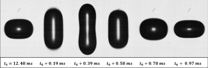
Figure 5. A typical cycle of the l = 2 mode beginning at t = 12.48 ms. The equilibrium bubble diameter is 0.43 mm.
Download figure:
Standard image
Figure 6. Shape mode analysis for the oscillating bubble in case 1. The left column shows even coefficients, from top to bottom, (a) b2, (b) b4 and (c) b6. The right column shows (d) odd coefficients b1, b3, b5, (e) volume mode coefficient b0 and (f) the normalized volume calculated using equation (9).
Download figure:
Standard imageThe volume mode, b0, shown in figure 6(e), also oscillates at the applied frequency but is negative. Figure 6(f) shows that the volume is approximately constant throughout the oscillation, indicating that the growth of the even modes (b2, b4, b6) is exactly countered by the contraction of the volume mode, b0. From this one can speculate that the field strength is too small to provide the thermodynamic work necessary to expand the bubble. Further discussion of this effect follows in section 5.2.
4.2. Case 2: oscillations of the l = 4 mode
As observed in section 4.1, the l = 2 mode is dominant for a broad range of frequencies and can be strongly excited even when f/f2 ≠ 1. The nonuniformity of the applied field allows the possibility of higher order modes, which will appear when the pressure frequency, f, approaches the higher mode frequencies determined by (6) and (7). As we increase the applied frequency well above f2 and approach f4, we observe visual evidence of the l = 4 mode. In the next example, the applied frequency remains the same (500 Hz) but the bubble radius is increased to 0.32 mm, resulting in higher relative frequencies, f/f2 = 1.25 and f/f4 = 0.45. Figure 7 shows the applied voltage, current, and normalized pressure. The driving pressure signals are very similar to figure 4, except that the Weber number is now lower. Figures 8 and 9 show, respectively, a typical oscillation cycle for case 2 and the shape mode analysis. A close look at figure 8 reveals that the l = 4 mode is present and superimposed over the still dominant l = 2 mode. It was observed that neither an increase in the frequency (such that f/f4 ∼ 1) nor an increase in the electric field pressure resulted in a case where the l = 4 was dominant. This indicates the strong role that field geometry and symmetry play in the excitation of these modes. The approximately uniform field will always excite the l = 2 mode to some degree. To isolate the l = 4 mode, a different field geometry is required. Work by Bellini [27] indicates that a quadrapole field configuration would be optimal due to its particular form of symmetry.

Figure 7. The applied voltage, current and normalized electric field pressure used to drive l = 4 oscillations of the levitated bubble in case 2.
Download figure:
Standard image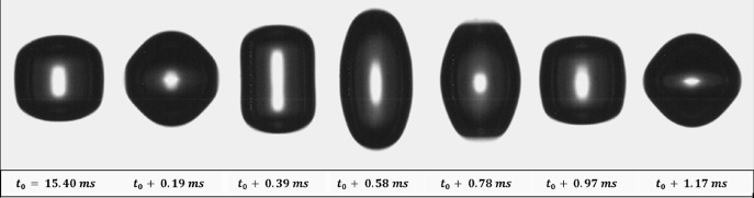
Figure 8. The l = 4 mode is observed to be superimposed on the usual l = 2 mode oscillation. The oscillation cycle begins at t = 15.40 ms. The equilibrium bubble diameter is 0.65 mm.
Download figure:
Standard image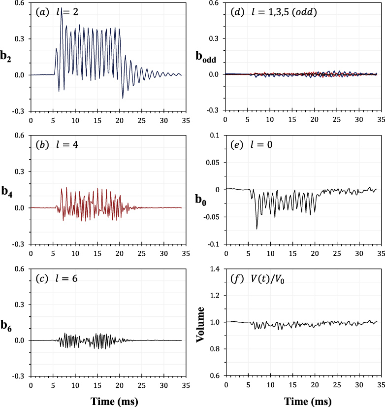
Figure 9. Shape mode analysis for the oscillating bubble in case 2. The left column shows even coefficients, from top to bottom, (a) b2 (b) b4 and (c) b6. The right column shows (d) odd coefficients b1, b3, b5, (e) volume mode coefficient b0 and (f) the normalized volume calculated using equation (9).
Download figure:
Standard image5. Implications for breakdown
5.1. Evaluating the shape effect
A key motivation, stated in section 1, for driving bubbles with an electric field was to explore the accompanying field enhancement due to shape distortions; this was defined as the shape effect. Enhancement of the field in this manner could reduce the voltage required to form electrical discharges inside a bubble and subsequently aid in the excitation of plasma discharges for water based applications. This field enhancement is a consequence of the permittivity gradient at the gas–liquid boundary. The shape of the boundary, and hence the shape of the bubble, ultimately determines how the external applied field is distributed within the bubble. To clarify, let us consider a second example: the ellipsoid in a uniform field. For simplicity, let the ellipsoid's major axis (along z) coincide with the applied field
and let the two perpendicular axes be equal. The ellipsoid is therefore axisymmetric about the applied field and its surface is defined by the following equation,

One can show that the electric field inside the ellipsoid is uniform and proportional to the applied field [20]. It can be calculated as a function of the aspect ratio of the ellipsoid, c/a, the permittivity of the ellipsoid, ε1, and the permittivity of the surrounding medium, ε2. Figure 10 shows values for the electric field in the ellipsoid for the case of a gas bubble in water. The field values are normalized to the applied field
. Let us refer to this normalized value as the enhancement factor, represented by G.
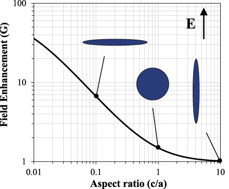
Figure 10. The electric field enhancement inside an axisymmetric ellipsoid air bubble. c and a represent dimensions parallel and perpendicular to the field respectively. From left to right, the displayed shapes represent c/a = 0.1, 1 and 10.
Download figure:
Standard imageFor large values of c/a, the bubble resembles a thin, long needle aligned with the field. In this case, the enhancement factor approaches unity and the internal field is equal to the applied field. For small values of c/a, the bubble is compressed into a thin flat disc. As c/a → 0, G can be shown to asymptotically approach ε2/ε1 [20], which for a bubble in water is 80. Although this would result in large amplification of the field, it would require an extreme aspect ratio. To obtain G = 70, for example, requires c/a = 1/1000. The extension and compression of ellipsoids, like those shown in figure 10, are similar to l = 2 shape oscillations. Since most of the observed bubble oscillations are dominated by the l = 2 mode, figure 10 can serve as a guide for studying the field distribution inside experimentally observed bubbles.
We begin the analysis of experimental data by considering four characteristic bubble shapes, shown in figure 11. These shapes represent the most extreme examples of the two most dominant modes observed. The first two frames show the l = 2 mode at (a) b2 = −0.424 and (b) b2 = 0.683. The next two frames show the l = 4 mode at (c) b4 = −0.101 and (d) b4 = 0.067. As described in section 4.2, the l = 4 mode was difficult to excite in isolation, and therefore exhibited less severe distortion. To better understand the relationship between shape distortion and internal electric field, we consider a scenario in which each of the four images in figure 11 are at rest in a uniform electric field, which is aligned along the vertical axis as shown. We employ a 2D version of the electrostatic solver Maxwell to solve for the field inside the bubble.
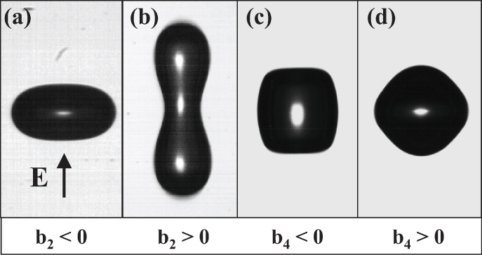
Figure 11. Four examples illustrating large excitation of the two dominant modes, (a) b2 = −0.424, (b) b2 = 0.683, (c) b4 = −0.101 and (d) b4 = 0.067. The applied field was oriented as shown.
Download figure:
Standard imageIn each case, the discrete spherical harmonic fit obtained through (5) was used to specify the shape boundary. The conductivity and relative permittivity of the water were set at 20 µS m−1 and 80 respectively, both chosen to replicate the experimental conditions. Solutions were arrived at with an energy error of less than 0.005% within 20–22 mesh iterations. The computed electric field distributions are shown in figure 12, with all values normalized to the external applied field. These values represent the position dependent enhancement factor inside the bubble, namely,
 . As a reference, define G0 to be 1.5, the enhancement for an unperturbed sphere.
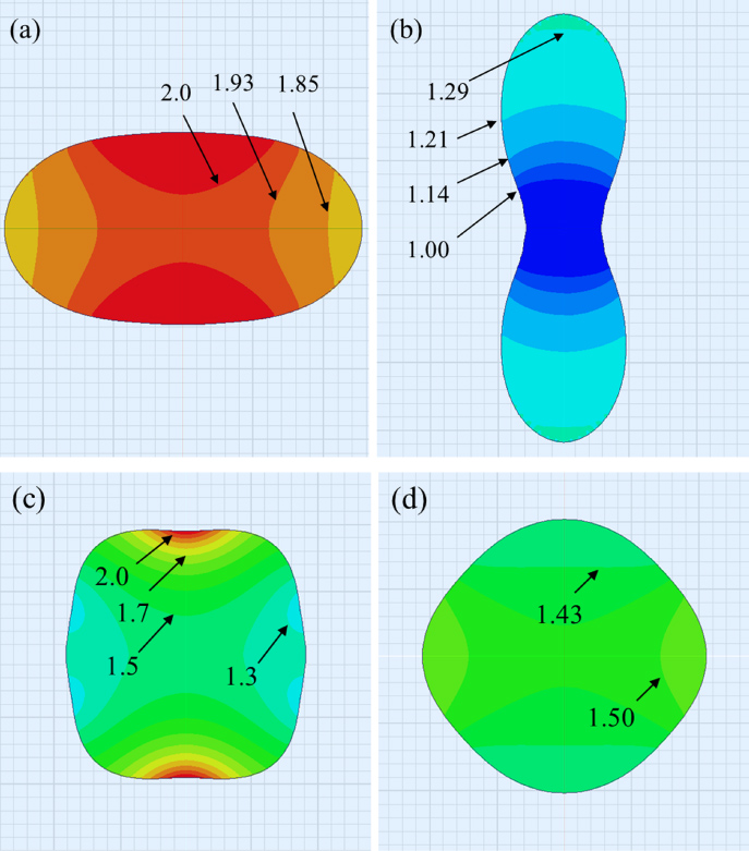
Figure 12. The enhancement factor G calculated for the four characteristic images in figure 12. The value G0 = 1.5 corresponds to the field in a sphere. Labels indicate the value of G at the boundary between two regions.
Download figure:
Standard imageThe two l = 2 mode examples are shown in (a) and (b). For b2 < 0, the field magnitude was enhanced above G0, with a maximum of 2.3 at the top and bottom ends. In contrast, for b2 > 0, the field was depressed below G0, with a maximum field of 1.3 at the axial ends and a minimum field of 1.0 at the centre of the bubble. This trend matches well with the ellipsoid from figure 10, in which compression of the bubble resulted in field enhancement while elongation resulted in field reduction. The primary deviation from the ellipsoidal shape is the localized contraction of the bubbles sides for b2 > 0. However, this local contraction does not appear to produce any appreciable distortion of the field.
The cases of (c) b4 < 0 and (d) b4 > 0 are shown in the bottom row of figure 12. The smaller deviation of G in these cases can be attributed to the small values of b4. Nonetheless, these results indicate a pattern that is similar to the case of l = 2; the negative coefficient results in field enhancement while the positive coefficient results in field reduction. The largest field enhancement, for b4 < 0, occurs at the axial ends and is 2.1. The lowest magnitude occurs for b4 > 0 and is 1.4. Despite the experimental observation of significant mode excitation for both l = 2 and l = 4, the resulting field distortion does not appear to be enhanced more than 53% above the baseline value of the sphere, G0.
Overall, the highest enhancement occurs when the bubble diameter contracts in the direction of the applied field. Expanding upon this observation, one can speculate that for large negative values of b2 and b4 (see figure 1), the field enhancement might be more extreme. We can calculate the theoretical enhancement for such extreme cases using a similar procedure. We consider stationary bubbles in a uniform field, now deformed into pure modes like those shown in figure 1. We then alter both b2 and b4 separately to determine the field enhancement in the limit of severe distortion. To simplify the discussion, we look at only the axial field distribution along the centreline of the bubble (parallel to the applied field). In most cases, this is where the maximum field occurs. Figure 13 shows axial field profiles for the (a) l = 2 mode and (b) l = 4 mode, with the coefficient b2 or b4 labelled beside each curve. Each case begins at z = 0 the centre of the bubble, and extends axially along the centreline up to the bubble boundary, where the field experiences a sudden drop-off due to the permittivity jump from gas to liquid. The field immediately outside the bubble is well below the applied value, 1.0, but increases with distance away from the bubble and approaches 1.0 asymptotically. The dotted line represents the case of the sphere, in which b2 and b4 are zero. As expected the enhancement inside the sphere is uniform and equal to 1.5. The simulations in figure 13 appear to be consistent with those in figure 12. When either coefficient b2 or b4 is positive, the field is predominantly lower than G0. As both coefficients become more negative, the air gap within the bubble contracts and the field becomes amplified far above G0. In the extreme case of b2 = −0.8, the bubble contracts to 20% of its original radius and has a maximum field enhancement of G = 50 near the edge of the bubble. This result is intuitive if one thinks of the bubble as an electrode gap: decreasing the electrode gap increases the approximate voltage drop per unit length.
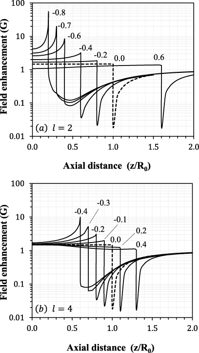
Figure 13. Axial electric field profile inside a gas bubble subjected to excitations of the (a) l = 2 mode and (b) l = 4 mode. The coefficient value, b2 or b4, is labelled beside each curve.
Download figure:
Standard imageOverall, figure 13 shows that for an electric field aligned with the bubble's axis of symmetry, large negative mode coefficients result in the strongest enhancement of the applied field. This enhancement is local and confined to small areas where the bubble's shape undergoes extreme contractions. Such contractions can result in the complete inversion of the water surface into a conic structure, closely resembling a sharp conducting tip (see figure 1). This localized behaviour can be contrasted with the ellipsoids presented at the beginning of section 5.1, which require physically impractical distortions of the shape to achieve comparable values of G. It is also clear that the orientation between the direction of bubble contraction and the applied field is important in obtaining field enhancement. In the case of figure 12(b), we observed that a contraction perpendicular to the field did not result in any field enhancement. Further simulations of the applied field orientation are required to determine the exact nature of this relationship.
The large field enhancement observed in figure 13 would require shape distortions more extreme than those achieved to date. In the future, it may be possible to obtain such levels of distortion by (1) increasing the applied electric field and (2) more carefully tuning the field frequency to the true resonance of each mode. This is complicated by the fact that, as mentioned in section 4, the resonance associated with nonlinear shape distortions does not match the linear modes given in equations (6) and (7). It has also been demonstrated, in the case of liquid drops [38, 39], that a sufficiently high field can destabilize the bubble, leading to the formation of extreme curvature surfaces and the expulsion of droplets. In both cases, a transient geometry of extreme curvature exists, which if combined with an applied electric field, may result in strong field amplification.
5.2. Evaluating the volume effect
The results from section 4 show that the applied field is not strong enough to alter the bubble's volume. This is because the ambient gas pressure, p0, is much larger than the surface tension stress, σ/2R0, and is therefore more difficult to overcome with a given value of electric field. For a 1 mm radius bubble, the ratio 2p0R0/σ is 2800, which means that even if the Weber number, We, were 4 (as in Case 1), the electric stress would still only be (4/2800) times as strong as the ambient pressure. In other words, even a 10% decrease in the gas pressure would require a field of at least 54 kV cm−1to sustain electrostatically. In theory, the electric field can be increased to sustain such large transient pressure changes in the bubble, but the high fields required may be too large to realize a positive effect from the distorting field. An alternative approach is to use acoustic pressure waves, which can be excited to the necessary ∼1 atm levels by using piezoelectric transducers similar to those discussed in section 2.1. Under these conditions, it has been predicted that large volume changes associated with the volume mode, b0, are achievable [40, 41].
6. Concluding remarks
The extreme distortion of gas bubbles can be used as a tool to facilitate plasma breakdown within bubbles submerged in water. This can be accomplished through two mechanisms: (1) the shape effect, in which distortions to the gas–liquid dielectric boundary act to enhance the local electric field and (2) the volume effect, in which the internal gas pressure of the bubble temporarily decreases due to an expansion of the bubble volume.
In this work, we have introduced a device capable of trapping air bubbles with an acoustic field and exciting them into strong, nonlinear shape oscillations using an ac electric field. Mode decomposition analysis of images taken using a high-speed camera indicates the presence of both the l = 2 and l = 4 spherical harmonic modes. Electrostatic simulation of the field inside these imaged bubbles indicates that the electric field is enhanced up to 53% higher than the case of a sphere. Furthermore, simulations show that an increased excitation of either the l = 2 or l = 4 mode may result in enhancement factors up to an order of magnitude higher (G = 10–50) than those observed empirically to date. It is clear that suitable demonstration of the volume effect will require either stronger electric fields or an alternative driving method. Overall, the true practically of both effects will be tested in future work by direct plasma ignition inside deformed gas bubbles.
Acknowledgments
This work was supported by the National Science Foundation (CBET 0939879).