

Abstract
We are reporting on analysis, design, construction, and key parameters of the device for a two-way time transfer via an optical fiber. The dominant source of errors in the two-way optical time transfer (TWOTT) via relatively short optical fibers is the temperature dependence of internal delays within the terminal units. We have performed an analysis of the influence of the internal delays and their temperature dependence on the TWOTT process considering two different configurations of the terminals with the feedback coupling in optical and electrical domains. The achieved results have been used for the optimal design of a TWOTT system implementing standard small form-factor pluggable optical transceivers. The operational tests of this new TWOTT system confirmed the precision of the time transfer on the subpicosecond level, the time transfer stability characterized by TDEV better than 60 fs for averaging intervals from 100 s to 10 000 s, and the temperature stability better than 100 fs K−1.
Export citation and abstract BibTeX RIS

Original content from this work may be used under the terms of the Creative Commons Attribution 3.0 licence. Any further distribution of this work must maintain attribution to the author(s) and the title of the work, journal citation and DOI.
1. Introduction
In contemporary space geodesy there are increasing requirements for accuracy of the time synchronization between different geodetic techniques, e.g. GNSS (Global Navigation Satellite System), SLR (Satellite Laser Ranging), and VLBI (Very Long Baseline Interferometry). The integration of multiple techniques in order to create the infrastructure necessary for monitoring the Earth system and for global change research is organized by GGOS (Global Geodetic Observing system). Considering the magnitude and rate of observed changes, the most demanding goal of GGOS initiative is definition of station positions to an accuracy of 1 mm and the corresponding velocities to 0.1 mm yr−1 with respect to ITRF (International Terrestrial Reference Frame). The integration of multiple techniques requires synchronization of their time scales with accuracy at least comparable with accuracy of the geodetic measurements. Therefore the accuracy should be near one picosecond.
In the past, a lot of effort went into the development of a very precise Two-Way Time Transfer (TWTT) using a coaxial cable as the transmission link [1] with the aim to identify unaccounted system delays at the Geodetic Observatory Wettzell. The main disadvantage of this approach is a rather steep increase in the time transfer error with the length of the link due to the propagation loss at high frequencies. It provides good results for links of the length up to several hundred meters, but for distances of several kilometers accuracy better than 100 ps cannot be expected even though high performance cable is used.
This limitation can be resolved by using optical telecommunications technology. In recent years, we can observe rapid progress in the field of time and frequency transfer via optical fibers. Notable results have been already achieved even with relatively long optical links [2–7]. Some of these projects are dealing with a high performance optical frequency transfer [8–10], which is typically used for comparing optical frequency standards. However, in many applications high accurate time transfer is required as well [11–13]. In cases where slightly subnanosecond accuracy is sufficient, the time transfer can be solved using the popular White Rabbit technique [14], but in other cases like the fundamental geodesy the accuracy requirements are much more severe.
With the aim to enlarge the area where time transfer with picosecond accuracy can be ensured, we started to work on a new Two-Way Optical Time Transfer (TWOTT) system implementing standard small form-factor pluggable (SFP) optical transceivers to transfer timing information between two or more terminals. The advantages of the economical solution based on the standard SFPs for the TWOTT have been already proved in past projects [15–18].
We focused on the potential applications where comparisons of two or more clocks deployed in a relatively small area are required. These cases are typically observatories and large laboratory campuses where the typical length of the optical links is not longer than several kilometers. Thanks to this limitation, we do not need to consider effects like the fiber chromatic dispersion, large link attenuation, and relativistic effects [19], which play important roles in the TWOTT on very large distances.
On the other hand, when relatively short fibers are considered and the above-mentioned effects can be neglected, the dominant source of systematic measurement errors will be the temperature dependence of internal delays within the TWOTT terminal units. The TWTT technique [20] perfectly eliminates the influence of the large link delay including its variations, but it does not suppress the impact of some partial internal delays within the terminal units. These internal delays are usually not greater than several nanoseconds. They are relatively small, but not negligible, and their dependence on temperature can be a source of an unpleasant error and instability in the time transfer. Therefore, the key goal of the design of a very precise TWOTT system is keeping the impact of these effects as low as possible.
We have performed a detailed theoretical analysis of the influence of the partial internal delays and their temperature dependence on the TWOTT process. We investigated two different configurations of the TWOTT terminals with the feedback coupling in optical and electrical domains. The results of the analyses have been experimentally proved for both considered cases. Afterward, the achieved results have been used for the optimal design of the TWOTT system.
2. Two-way time transfer analysis
We will analyze the TWTT process with the aim to investigate the influence of the partial delays within the TWTT units on the resulting error of the time transfer. For the purpose of the analysis we consider the general setup of the TWTT system shown in figure 1. It consists of two units, A and B, interconnected by a transmission link. Each of the units includes a timing signal generator and an event timer, which measures times of arrival of timing signals coming to its input. The output of the timing signal generator and the input of the event timer are connected to the transmission link via a network consisting of five branches connected in three splitters/couplers. This network provides feedback coupling of the transmitted signals back to the event timer and the bidirectional use of the transmission line. The branches in the networks have delays  ,
,  ,
,  ,
,  ,
,  and
and  ,
,  ,
,  ,
,  ,
,  . The transmission link has delay,
  .
.

Figure 1. General setup of the TWTT system consisting of two units, A and B, connected by a transmission link. Each unit includes a timing signal generator, TSG, and an event timer, ET. The output of the generator and the input of the event timer are connected to the transmission link via a network consisting of five branches and three splitters/couplers which provide feedback of the transmitted signals to the event timer and the bidirectional use of the transmission line. Each of the branches represents a chain of opto-electronics and/or interconnection lines.
Download figure:
Standard image High-resolution imageEach of the branches represents a chain of opto-electronics and/or interconnection lines. The form of the individual branches depends on the arrangement of the units used in the particular TWTT system. Two basic concepts of the unit for TWOTT are shown in figures 2 and 3. The first uses the feedback coupling in the electrical domain, i.e. the generated timing signal is branched off to the event timer before it is converted to the optical signal. The second is based on feedback coupling in the optical domain. In this case, the generated timing signal is first converted into an optical signal and then branched off to the input of the optical receiver where it is processed like the signal received from the transmission link.

Figure 2. TWOTT unit with feedback coupling in electrical domain.
Download figure:
Standard image High-resolution image
Figure 3. TWOTT unit with feedback coupling in optical domain.
Download figure:
Standard image High-resolution imageEach of the units uses its own local time scale for the time of arrival measurements. In the analysis we consider that the time scale A is delayed by  with respect to the time scale B. The goal of the time transfer is to determine the time difference
  between both time scales.
The time transfer process is initiated at the time  when the unit A generates a timing signal. The signal propagates to the event timers in both units. After it arrives, the event timer A records the time of arrival:

and the event timer B records the time of arrival:

In the second step, unit B generates a timing signal at the time  . In this case, event timer A records the time of arrival:

and event timer B records the time of arrival:

The desired time difference can be expressed from the measured times of arrival:
In real cases the exact values of the internal delays are not known, and we must be satisfied with the time difference estimation:
which is based on the assumption:

thus this estimation is affected by an error:
Evidently, the error will be zero when we ensure perfect symmetry of the internal delays in both units, i.e.  ,
,  ,
,  ,
,  . Often, it is impossible to meet such a requirement with acceptable accuracy and the error must be eliminated by means of a common clock calibration.
Besides the time transfer we can also get the delay of the transmission link:
or rather its estimation:

In this case, the error of the estimation is:

and cannot be simply eliminated on the basis of the symmetry of the internal delays in the units.
From the point of view of keeping good temperature stability of the time transfer, it is important to know the sensitivity of the time transfer results on changes of the internal delays. The sensitivity of the time difference and link delay estimations to the change of the temperature in the unit A are:
and the sensitivity to the change of the temperature in the unit B are:
The largest temperature dependence of the delay can be expected in the optical transmitter and the optical receiver, which include relatively complex electronics unlike the electrical and optical interconnections formed by passive links. Therefore, the branches including the optical transmitter and receiver are dominant sources of the temperature dependence and the other branches can be usually neglected.
In the optical TWTT unit with feedback coupling in the electrical domain (see figure 2), the optical transmitter is situated in branch 2 and the optical receiver in branch 5. If the temperature coefficients of the delays in these branches are replaced by the temperature coefficients of the delays of the optical transmitter and the optical receiver  and
and  , respectively, and the temperature dependences of the other delays are neglected, the approximations of the resulting temperature coefficients are:
In the TWOTT unit with feedback coupling in the optical domain (see figure 3), the optical transmitter is situated in branch 1 and the optical receiver in branch 4. Therefore the resulting temperature coefficients can be approximately expressed:


The conclusion from the previous is that the temperature dependence of the TWOTT using feedback coupling in the electrical domain is mostly given by the difference of the temperature dependences of the optical transmitter delay and the optical receiver delay. On the other hand, the temperature dependence of the optical time transfer with feedback coupling in optical domain is approximately equal to the temperature dependence of the optical receiver delay.
3. Experimental setup
The experiments have been performed on an in-house developed TWOTT system based on standard small form-factor pluggable (SFP) optical transceivers. The single mode SFPs were operated at the wavelength of 1550 nm.
The system allows the time transfer between two or more terminals (see figure 4). Two terminals are simply interconnected by a fiber. When three or more terminals are involved in the system, optical splitters are employed in the fiber infrastructure (see figure 5). The objective of the time transfer is to compare time scales represented by a 1PPS time mark and a 100 MHz frequency reference. These signals generated by external clocks are connected to each of the terminals. The TWOTT terminals make it possible to use the feedback coupling both in the optical domain and the electrical domain.

Figure 4. The inside of the TWOTT terminal. In front, from left to right, there are the event timer, the TWTT board, and optical splitters.
Download figure:
Standard image High-resolution image
Figure 5. When three or more terminals are involved in the system, optical splitters are employed.
Download figure:
Standard image High-resolution imageA proprietary communication protocol has been implemented in the TWOTT system to ensure proper communication between the terminals. One of the terminals is designated as a Master, while the others are Slaves. The Master manages the operation of the entire system.
The sharing of the optical link by two or more TWOTT terminals is based on Time Division Multiple Access (TDMA). The TDMA frame of the length of 1 s is divided into 10 time slots of the length of 100 ms which are allocated to individual terminals. The allocation scheme depends on the number of terminals sharing the optical link. In figure 6, there is the TDMA scheme for the simplest case when the Master keeps communication with the only Slave. The slot number 5 is always reserved for measuring times of arrival of the external 1PPS. Therefore, this slot is centered at integer seconds of the external time scale connected to the Master terminal. This time scale serves as the system time used for the synchronization of operation of all terminals in the system. The time scales connected to other terminals can differ from this system time not more than 50 ms.

Figure 6. Time division multiple access (TDMA) pattern used for TWOTT between two terminals.
Download figure:
Standard image High-resolution imageIn each allocated slot, the terminal sends 45 timing signals and the data messages necessary for TWOTT system operation. To avoid a DC component in the waveform, the data are encoded using the Manchester code. The bit rate of the data transmission is 50 Mb s−1.
The timing signal is represented by a 16-bit pseudorandom sequence. On the basis of its detection, the control logic of the terminal opens a gate, which selects the next rising edge out of the received signal forming a pulse, which is time tagged by the event timer with respect to its local time scale based on the external frequency reference of 100 MHz. Thanks to the use of a new event timing technique [21–26], the times of arrival can be measured with subpicosecond precision, thus the influence of the event timer on the resulting TWOTT precision is negligible.
From the times of arrival collected in the 1 s TDMA frame, the resulting time difference between the time scales (Slave-Master) is computed:

where  (
( =
=  ,
,  ,
,  ,
,  ) is a vector of times of arrival of timing signals sent by the terminal
  measured by the event timer in the terminal
  ,
,  (
( =
=  ,
,  ) is the time of arrival of the 1PPS time mark measured by the event timer in the terminal
  , and the operator
  stands for the determination of the fitted value at the integer second of the system time (the mid of the slot 5) using linear fit.
Although the external time scale and the local time scale used by the event timer are based on the same frequency reference, the difference between the time scales can slightly change because of the temperature dependence of the delays of the distribution paths. Since these changes are very slow, the times of arrival of the 1PPS time marks can be effectively filtered. This allows suppression of the 1PPS jitter, which is usually significant in comparison with the TWOTT precision.
During the experiments, 1PPS time marks with a slew rate of 5.7 V ns−1 were split into both terminals (see figure 7). These time marks were generated directly from the 100 MHz frequency reference used in both terminals. The terminals were interconnected with a single mode optical fiber 20 m in length. The interconnection coaxial cables were not longer than 2 m. The setup was installed in a common laboratory environment with relatively stable temperature (±0.5 K).
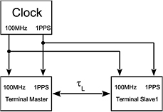
Figure 7. Common clock experimental setup. The same 1PPS time marks and 100 MHz frequency reference were connected to both TWOTT terminals.
Download figure:
Standard image High-resolution image4. Measurement of temperature dependence
The model of the sensitivity of the TWOTT to a temperature change has been verified in a common clock experiment. We kept the temperature stabilized in both terminals and then we changed the temperature by approximately 6 K in the Master terminal. After the temperature was steady again, we changed the temperature in the Slave terminal. The length of the temperature transitions was around 30 min. The temperatures inside the terminals were measured using built in temperature sensors situated inside the SFPs. We performed this experiment both for the optical and electrical feedback coupling.
The temperature coefficients of the resulting time difference and of the link delay estimations were determined from their responses to the relatively slow temperature changes by linear fits. The results are summarized in tables 1 and 2. The temperature coefficients of the receiver delay and of the transmitter delay presented in the tables were estimated from the simplified models of the temperature dependence (20)–(30) for the optical feedback coupling, and (16)–(19) for the electrical feedback coupling.
Table 1. Temperature coefficients of TWOTT using optical feedback coupling.
| Temperature coefficients | Master (ps K−1) | Slave (ps K−1) |
|---|---|---|
| Time difference | −1.28 | 1.42 |
| Link delay | 0.19 | 0.13 |
| Receiver delay | 1.28 | 1.42 |
| Transmitter delay | — | — |
Table 2. Temperature coefficients of TWOTT using electrical feedback coupling.
| Temperature coefficients | Master (ps K−1) | Slave (ps K−1) |
|---|---|---|
| Time difference | −0.59 | 0.52 |
| Link delay | 0.87 | 1.06 |
| Receiver delay | 1.46 | 1.58 |
| Transmitter delay | 0.28 | 0.54 |
When the optical feedback coupling was used, the temperature dependence of the link delay results were much lower in comparison to the temperature dependence of the time difference results. It is in agreement with the theoretical model, which supposes that the temperature dependence of the link delay results is near zero, while the temperature dependence of the time difference results are fully determined by the temperature dependence of the optical receiver. The temperature coefficients of the receiver delays computed from this measurement are both near 1.35 ps K−1. The temperature coefficients of the transmitter delays cannot be determined in this case because the measurement results do not depend on the transmitter delay.
When we used the electrical feedback coupling, the temperature dependence of the resulting time difference was considerably lower and the temperature dependence of the resulting link delay was much higher in comparison with the previous case. It is again in agreement with the theoretical model. The temperature coefficients of the receiver delays computed from these results are both near 1.50 ps K−1, which is not far from the previous results.
In the data messages transmitted between the terminals, in addition to the measured times of arrival, other parameters also included the temperature measured inside the terminals which can be used for a temperature correction of the TWOTT results. The necessary temperature coefficients must be determined on the basis of a calibration measurement before the terminals are used in the system. When the temperature correction is applied, better performance can usually be achieved using the optical feedback coupling, where the optical receiver is the only dominant source of the temperature dependence. When the temperature correction is not applied, better temperature stability can be expected using the electrical feedback coupling.
5. Tests of TWOTT system
The properties of the TWOTT system were evaluated in a series of common clock experiments. The feedback coupling in the optical domain was used during these experiments, i.e. the timing signal was first converted into the optical signal and then branched off to the input of the optical receiver and processed like the signal received from the transmission link.
The first experiment was focused on testing of the TWOTT performance under stable temperature conditions. The development of temperatures in both terminals during the 8 h measurement is shown in figure 8. The resulting time difference is shown in figure 9. Each point represents the result of a 1PPS time comparison. The line represents time difference estimations computed by a linear fit on consecutive 5 min intervals and related to midpoints of these intervals. The standard deviations of the individual 1 s comparisons and of the 5 min linear fits are 415 fs and 82 fs, respectively.

Figure 8. Development of temperatures in both terminals during 8 h measurement.
Download figure:
Standard image High-resolution image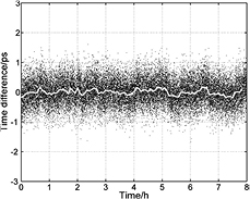
Figure 9. Resulting time difference during 8 h TWOTT measurement under stable temperature. Data are centered, i.e. average value was subtracted from all the data. Each point represents the result of an individual 1PPS time comparison. Solid line represents 5 min linear fits. Standard deviations of individual 1 s comparisons and of 5 min linear fits are 415 fs and 82 fs, respectively.
Download figure:
Standard image High-resolution imageThe time transfer stability characterized by TDEV computed from the results of the 1 s comparisons is plotted in figure 10. The TDEV curve is composed of three regions. In the first region, the TDEV follows the white phase noise slope up to averaging intervals of several tens of seconds. In this region the influence of the 1PPS time mark jitter is suppressed by filtering and the TDEV represents the optical time transfer noise only. On the other hand, in the third region, which starts around 1 h, the 1PPS jitter filtering is no longer effective and the TDEV represents mainly the 1PPS jitter, which is dominant with respect to the time transfer noise. In the transition region the TDEV is leveling around 50 fs.

Figure 10. Time transfer stability characterized by TDEV computed from the results of 1 s comparisons.
Download figure:
Standard image High-resolution imageUsing the same measurement data, we also assessed the performance of the TWOTT system in the regime when the external 1PPS time marks are fully omitted and the TWTT is used just for the frequency comparison of the external reference frequency sources. In this case, the 1PPS jitter has no influence on the frequency transfer precision and the precision is given only by the TWOTT performance. The resulting frequency transfer stability characterized by Allan deviation (ADEV) computed from the results of the 1 s comparisons is plotted in figure 11. The ADEV plot follows the white/flicker phase noise slope in the entire considered range of averaging intervals up to 10 000 s where the ADEV falls under  .
.

Figure 11. Frequency transfer stability characterized by Allan deviation (ADEV) computed from results of 1 s comparisons.
Download figure:
Standard image High-resolution imageIn the next experiment we introduced an intentional temperature change by 5 K inside the Slave terminal. The measured temperatures inside Master and Slave terminals during the 90 min experiment are plotted in figure 12. The resulting time difference without the temperature correction and with the temperature correction is plotted in figure 13. The temperature dependence coefficients without the correction and with the correction determined by linear fits are 1.38 ps K−1 and −0.08 ps K−1, respectively (see figure 14). The temperature correction was based on an independent calibration measurement performed six months before the experiment.

Figure 12. Temperature inside the Master (solid line) and Slave (dashed line) terminals during the test.
Download figure:
Standard image High-resolution image
Figure 13. Resulting time difference without temperature correction (solid line) and with temperature correction (dashed line).
Download figure:
Standard image High-resolution image
Figure 14. Resulting temperature dependence coefficients without temperature correction (solid line) and with temperature correction (dashed line) are 1.38 ps K−1 and −0.08 ps K−1, respectively.
Download figure:
Standard image High-resolution image
6. Conclusions
Two basic configurations of the TWOTT terminals with the feedback coupling in optical and electrical domains were analyzed with the aim to investigate the influence of the partial internal delays and their temperature dependence on the TWOTT process. The analyses demonstrate that the temperature dependence of the TWOTT using feedback coupling in the electrical domain is mostly given by a half of the difference of temperature dependences of the optical transmitter delay and of the optical receiver delay. On the other hand, the temperature dependence of the optical time transfer with the feedback coupling in optical domain is approximately equal to the temperature dependence of the optical receiver delay. The results of the analyses have been experimentally verified for both considered cases.
The achieved theoretical results have been used for the optimal design of a TWOTT system aimed at applications using optical links up to several kilometers in length. The properties of this system have been evaluated in a series of common clock experiments. The resulting standard deviation of the time transfer is 415 fs for 1 s comparisons, the standard deviation of 5 min linear fits is 82 fs, and the time transfer stability characterized by TDEV is better than 60 fs for the range of averaging intervals from 100 s to 10 000 s.
We also assessed the performance of the TWOTT system in the regime when it is used just for the frequency comparison of the external reference frequency sources. The resulting frequency transfer stability characterized by ADEV follows the white/flicker phase noise slope in the entire considered range of averaging intervals up to 10 000 s where the ADEV falls under  .
.
Finally we tested the temperature stability of the TWOTT, i.e. the response of the time comparison results to a change in the temperature of the terminal. Using a temperature correction based on a calibration performed several months ago, the sensitivity to the temperature change was kept lower than 100 fs K−1.
Acknowledgments
This work was partially supported by DFG project FOR1503 and ESA Contract No. 4000112251/14/NL/FC.