Particle-in-cell simulations of parametric decay instability of radiofrequency wave in the ion cyclotron range of frequency in an inhomogeneous plasma

The simulation model is shown in figure 1. We consider a slab model of tokamak plasma with the external magnetic field along the y (toroidal) direction, and the magnetic field and density gradient in the x (radial) direction. The z direction denotes the poloidal direction. The simulation length in the x direction is lx = 0.06 m. There is a vacuum region between the left boundary x = 0 m and the plasma edge x₀ = 0.0012 m. Since the plasma density profile is unavailable in the experiments, we assume it to be n(x) = n₀[0.43a tan (5x/lx − 2) + 0.47], as shown in figure 1, where n₀ = 2.0 × 10¹⁷ m⁻³. A perturbation current is placed in the vacuum with the expression J(x, t) = J₀exp(−(x − 0.0006)²/0.0006²) sin (ω₀t)(1−exp(−γt))², where γ = 0.02ω₀ and (1 − exp(−γt))² is a ramped factor used to avoid the excitation of the local modes [28]. The thin vacuum layer on the left edge is used to reduce the effect of particle perturbation on this current source. A pump wave with frequency ω₀ is launched and then propagates into the plasma. In the simulation, 900 particles per cell are typically used for the perturbation current amplitude J₀ = 2 × 10² A m⁻². These particles are loaded as the Maxwellian distribution in velocity space and uniformly in space. When the particles reach the left or right boundary, they are absorbed and removed from the simulation. Both electrons and ions are treated by a fully kinetic model. For simplicity, the plasma temperature is assumed to be uniform in the simulation region. The temperatures of the ions and electrons are 30 eV and 50 eV, respectively. Typically, the spatial grid resolution is Δx/ρ_i ≃ 0.08, which is high enough to resolve the ion gyro motion. The typical duration of our simulations is several hundred of rf periods, which brings us the high frequency resolution during the FFT and takes approximately 24 h with 64 cores on our cluster.

Zoom In Zoom Out Reset image size

From the linear theory, the launched electron plasma wave (EPW) propagates towards the cold plasma resonance layer and then transforms smoothly into the IBW in an inhomogeneous plasma, arising from the finite ion-Larmor-radius effect [9, 29]. The relevant electrostatic dispersion relation can be expressed as [9]

$$\begin{equation} K_{xx} =-\frac{\left| {K_{xy}} \right|^{2}}{{c^{2}k^{2}}/{\omega ^{2}}}-\frac{k_{\parallel}^{2} K_{zz}}{k_{\bot}^{2} -\left( {{\omega ^{2}}/{c^{2}}} \right)K_{zz}}, \end{equation} \tag{ 1 }$$

where K_xx,K_xy and K_zz are elements of the plasma dielectric tensor and can be written as

$$\begin{eqnarray} &&\fl K_{xx}\! =\!1+\frac{\omega_{pe}^{2}}{\Omega_{e}^{2}}\!+\!\sum\limits_j {\frac{\omega_{pj}^{2}}{\omega k_{\parallel} v_{tj}}\frac{\exp \left( {-b_{j}} \right)}{b_{j}}} \sum\limits_{m=1}^\infty {m^{2}I_{m} \left( {Z_{m} \!+\!Z_{-m}} \right)},\nonumber\\ &&\fl K_{xy} =-{\rm i}\frac{\omega_{pe}^{2}}{\omega \Omega_{e}^{2}}+{\rm i}\sum\limits_j {\frac{\omega_{pj}^{2}}{\omega k_{\parallel} v_{tj}}\exp \left( {-b_{j}} \right)} \sum\limits_{m=1}^\infty {m\left( {I_{m} -{I}'_{m}} \right)}\nonumber\\ &&\quad \times \left({Z_{m} -Z_{-m}} \right) ,\nonumber\\ &&\fl K_{zz} =1+\frac{2\omega_{pe}^{2}}{k_{\parallel}^{2} v_{te}^{2}}\left( {1+\zeta_{0e} Z_{0}} \right). \end{eqnarray} \tag{ 2 }$$

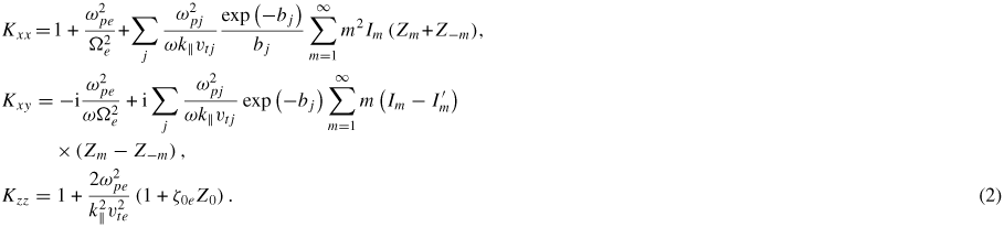
In equation (2), the summation j is over ion species, m is the harmonic number, Z_m is the plasma dispersion function with argument ζ_mα ≡ (ω + mΩ_α)/k_∥v_tα, $v_{t\alpha} \equiv \sqrt {{T_{\alpha}}/{m_{\alpha}}}$, α denotes species, and I_m is the modified Bessel function with argument $b_{j} \equiv {k_{\bot}^{2} v_{tj}^{2}}/{\Omega_{j}^{2}}$. The cold plasma resonance, which separates EPW and IBW regions, occurs when K_xx vanishes in the limit T_i = 0.

In order to reproduce this mode-transformation process, a plasma with single ion species (hydrogen) is taken into account. The density profile is kept the same as shown in figure 1 and the external magnetic field is uniform and B₀ = 1.2T. The injected frequency ω₀ = 1.77Ω_H. The ion gyroradius of hydrogen ρ_H = v_tH/Ω_H = 6.6 × 10⁻⁴ m and k_⊥ρ_H ≃ 0.8 at x = 0.02 m. With these parameters, the corresponding dispersion curve, i.e. the perpendicular wavenumber versus the radial position, is plotted as the blue solid line in figure 2(a). The cold plasma resonance layer locates at x = 0.009 m. The spatial distribution of E_x for the driving frequency from the simulation is illustrated in figure 2(b). It shows that the launched EPW transforms to an IBW and then penetrates into the plasma interior. The perpendicular wavenumber k_⊥ calculated from the simulation is compared with the linear dispersion curve, and excellent agreement is shown in figure 2(a). The frequency spectrum of the wave amplitude |E_x| in figure 2(c) indicates that only the peak of the driving frequency appears, and no sideband is present.

Zoom In Zoom Out Reset image size

For a low incident rf power, our simulation provides the mode converted electrostatic IBW as predicted by the linear theory. Good agreement in the comparison justifies our simulation model.

To investigate the PDI process, we raise the perturbation current amplitude to J₀ = 6 × 10² A m⁻² and the obtained electric field is about several 10⁴ V m⁻¹, which is close to that observed in the experiment. While other parameters are kept the same as in the above case, the second harmonic of the pump wave is observed in the simulation. The spatial distributions of E_x for the pump and second harmonic waves at different times are shown in figure 3. Clearly, the second harmonic wave is generated around the place x = 0.02 m.

Zoom In Zoom Out Reset image size

In order to explain the generation of the second harmonic wave, we plot the linear dispersion curves of the injected frequency and its second harmonic in figure 4 as the blue solid line and black dashed–dotted line, respectively. It is shown that the selection rule $2k_{\omega_{0}} =k_{2\omega_{0}}$ for the resonant mode–mode coupling can be satisfied at x ≃ 0.02 m (indicated as the vertical magenta dashed–dotted line). This suggests that the second harmonic wave could be resonantly excited. The wavenumbers of the pump wave and its second harmonic are compared with the linear dispersion relation of IBWs in figure 4. Good agreement in the comparison shows that the second harmonic wave is an IBW generated by the resonant PDI process.

Zoom In Zoom Out Reset image size

It is also noticed that the selection rule $k_{\omega_{0}} +k_{2\omega _{0}} =k_{3\omega_{0}}$ can be matched at x ≃ 0.026 m (indicated as the vertical cyan dash line in figure 4). One would expect the third harmonic wave to be excited if the amplitudes of the pump and the second harmonic waves are large enough. Such three-wave interaction is indeed observed in the simulation. Figure 5 illustrates the contours of the amplitude of |E| in the x − ω plane at different times from the simulation. In figure 5(a), one can see that the pump wave is generated and propagates into the plasma. As time goes on, the second harmonic wave appears around x = 0.02 m (indicated by the vertical magenta dashed–dotted line) where $k_{2\omega_{0}} =2k_{\omega _{0}}$ and its amplitude increases (figures 5(b) and (c)). As shown in figure 4, the group velocity of the second harmonic wave is very small near the resonant region. Thus the second harmonic wave propagates slowly in this region. Later on, as both the pump and second harmonic waves pass through the position x = 0.026 m (indicated by the vertical cyan dashed line), where $k_{\omega_{0}} +k_{2\omega_{0}} =k_{3\omega_{0}}$, a weak third harmonic wave is excited (figure 5(d)) and then propagates into the plasma (figures 5(e) and (f)).

Zoom In Zoom Out Reset image size

A comparison of the frequency spectrum between our simulation result and the experimental observation is displayed in figure 6. One type of wave spectrum measured on the HT-7 tokamak during an IBW heating experiment [17], illustrated in figure 6(a), shows that the peaks of the half (f_D), second (f_2H) and third (f_3H) harmonics of the pump (f₀) were observed. In the wave spectrum obtained from the simulation (figure 6(b)), the waves with the frequencies of the pump (ω₀), second (2ω₀) and third (3ω₀) harmonics are also found. The half-pump frequency is absent because the simulation parameters (for instance, the density and temperature profiles) are not exactly the same as those in the experiment. In the simulation, the matching condition $k_{\omega_{0}} =2k_{0.5\omega _{0}}$ is satisfied at the place x = 0.008 m where the amplitude of the pump wave is too small to drive the nonlinear PDI process. The simulation result indicates that the generation of the second harmonic mode is due to the resonant self-interaction of the incident wave as discussed in [24], while the excitation of the third harmonic mode is from the resonant mode–mode coupling between the pump wave and the generated second harmonic wave. Meanwhile, the zero-frequency mode $(\omega_{0} -\omega_{0} =0,k_{\omega_{0}}-k_{\omega_{0}}=0)$ is also produced in figure 6(b), which was also observed in [30].

Zoom In Zoom Out Reset image size

In the above case, the harmonics of the half-pump frequency wave do not appear in our simulation, while they have been observed in the experiments. In order to explore the generation of these modes, we change some of the plasma parameters to ensure the relevant selection rules can be satisfied in the simulation region. We consider a deuterium plasma with hydrogen minority and set the hydrogen concentration H/(H+D) = 0.15. The density profile is n(x) = n₀[(x − x₀)²/lx²] with n₀ = 2.5 × 10¹⁷ m⁻³ and the magnetic field varies along the x direction with the form B(x) = 1.57/(1.26 − x) T. The injected frequency is in the range of ω₀ = (1.70 ∼ 1.62)Ω_H and the ratio ω₀/Ω_H = 1.67 at x = 0.023 m.

The dispersion curves of this case for the driving frequency ω₀ and its half-harmonics 0.5ω₀ and 1.5ω₀ are plotted in figure 7. It shows that the selection conditions $k_{\omega_{0}} =2k_{0.5\omega_{0}}$ and $k_{\omega_{0}} =k_{1.5\omega_{0}} -k_{0.5\omega_{0}}$ are satisfied around x ≃ 0.023 m. It is implied that the waves with frequencies 0.5ω₀ and 1.5ω₀ could be produced by the resonant parametric decay if the amplitude of the pump wave is large enough.

Zoom In Zoom Out Reset image size

Figure 8 illuminates the history of the spatial variation of E_x for the pump wave and its half-harmonic. It is demonstrated that initially the half-pump frequency wave is present in the vicinity of the resonance layer. Later in time, the half-pump frequency wave grows and propagates into the plasma. The wavenumber of the half-pump frequency wave calculated from the simulation is dotted as the green triangles in the dispersion relation shown in figure 7, and it agrees well with the linear theory. Good agreement in the comparison confirms that the half-pump frequency wave is an IBW generated by the resonant PDI process.

Zoom In Zoom Out Reset image size

Figure 9 shows the comparison of the wave spectrum between the simulation and the experiment on the HT-7 tokamak [17]. In figure 9(a), a typical wave spectrum of PDI during IBW heating experiment on HT-7 [17] is illustrated. Obviously, the second harmonics (f_2H) and the harmonics of the half-pump frequency, including 0.5f₀, 1.5f₀ and 2.5f₀ (indicated as f_D, f_3D and f_5D), were detected in the experiment. The frequency spectrum of |E_x|²in figure 9(b) indicates that waves with the frequency of ω₀, 0.5ω₀, 1.5ω₀ and 2ω₀ are also generated in our simulation. Similarly, the wave with frequency 2.5ω₀ does not appear due to the mismatch of the k-matching condition. Our simulation result suggests that the half-harmonics of the pump wave are generated by the resonant mode–mode coupling. These resonant parametric decays are observed near the layers where the selection rules of mode–mode coupling are satisfied in inhomogeneous plasmas. If the selection rules are not satisfied, the corresponding waves are not observed in the simulations.

Zoom In Zoom Out Reset image size

In addition to the resonant parametric decay described in the previous subsection, nonresonant decay processes were also observed in the IBW heating experiments on the HT-7 tokamak [17]. To show these nonresonant PDI processes, we choose plasma parameters that remove all the resonant decay channels depicted above. The plasma density profile is kept the same as in the half-harmonics case while we set n₀ = 2.0 × 10¹⁷ m⁻³. The magnetic field is raised up a bit as B(x) = 1.93/(1.53 − x) T. The injected frequency is ω₀ ≈ 1.25Ω_H. The hydrogen concentration is set to H/(H + D) = 0.2 in this case. From the linear dispersion curves, second and third harmonics and half-harmonics frequencies cannot be resonantly generated in this case. We focus on the nonresonant mode–mode coupling in this subsection.

The time evolution of the contours of |E| in the x − ω plane (top) and normalized kinetic energy of deuterium (bottom) in the simulation are shown in figure 10. Figure 10(b) illustrates that the ICQM of D with frequency Ω_D ≃ 0.4ω₀ (marked as the white dashed–dotted horizontal line) and the corresponding beat wave with frequency 0.6ω₀ ≃ 1 − Ω_D (marked as the white dashed horizontal line) are excited near the cold plasma resonance layer at t = 397/ω₀. Simultaneously, the ion heating is significant at those places (figure 10(d)). However, ICQMs do not appear and no ion heating is observed in the resonant decay processes discussed above. Thus we believe that the ion heating might be caused by the heavily damping ICQMs produced by the nonresonant PDI process. Obviously, the energy of the pump wave will strongly deposit at the plasma edge due to the nonlinear Landau damping.

Zoom In Zoom Out Reset image size

In the above case, we show that only one nonresonant decay channel appears in the simulation. However, different decay channels may be excited simultaneously as observed in the experiments. For given plasma parameters, decay channels with the growth rate exceeding its damping rate will grow and compete with each other. Figure 11 illuminates an example that several decay channels coexist in the same time. In this case, the density profile is n(x) = n₀[0.37a tan (10x/lx − 4) + 0.49] with n₀ = 7.5 × 10¹⁶ m⁻³ and the other parameters are kept the same as the half-harmonics case. The selection rule $k_{\omega_{0}} =2k_{0.5\omega_{0}}$ can be matched in this case. The figure shows that the peaks of 0.4ω₀ = ω₀ −Ω_H (the beat wave between the injected wave and ICQM of H), 0.5ω₀ and 0.7ω₀ = ω₀ − Ω_D (the beat wave between the injected wave and ICQM of D) are observed. The corresponding ICQMs (Ω_H = 0.6ω₀ and Ω_D = 0.3ω₀) may be heavily damped on the ions and are absent in the frequency spectrum. Both H and D ions heating are found in this case.

Zoom In Zoom Out Reset image size