


Abstract
Several important ELM control techniques are in large part motivated by the empirically observed inverse relationship between average ELM energy loss and ELM frequency in a plasma. However, to ensure a reliable effect on the energy released by the ELMs, it is important that this relation is verified for individual ELM events. Therefore, in this work the relation between ELM energy loss  and waiting time
  is investigated for individual ELMs in a set of ITER-like wall plasmas in JET. A comparison is made with the results from a set of carbon-wall and nitrogen-seeded ITER-like wall JET plasmas. It is found that the correlation between WELM and
  for individual ELMs varies from strongly positive to zero. Furthermore, the effect of the extended collapse phase often accompanying ELMs from unseeded JET ILW plasmas and referred to as the slow transport event (STE) is studied on the distribution of ELM durations, and on the correlation between WELM and
  . A high correlation between WELM and
  , comparable to CW plasmas is only found in nitrogen-seeded ILW plasmas. Finally, a regression analysis is performed using plasma engineering parameters as predictors for determining the region of the plasma operational space with a high correlation between WELM and
  .
.
Export citation and abstract BibTeX RIS
This article was updated on 12 August 2021 to correct the copyright line.
1. Introduction
Standard high confinement (H-mode) regimes in tokamaks are characterized by the existence of an edge transport barrier (ETB) (typically called pedestal) in a narrow edge region inside the separatrix. Steep pressure gradients in the ETB lead to magnetohydrodynamic (MHD) instabilities called the edge-localized modes (ELMs) [1, 2]. ELMs are intense, short duration, repetitive events that cause a partial collapse of the ETB and result in sudden expulsion of energy and particles from the plasma edge. On the one hand, ELMs pose a serious concern as they can cause high transient heat loads on the plasma-facing components (PFCs) [3]. On the other hand, they are crucial for regulating the core concentration of impurities, in particular, tungsten (W), which is produced by plasma- wall interactions at the divertor target. Paradoxically, ELMs are required for impurity flushing even though they are responsible for at least a fraction of the W production in H-mode plasmas. Larger ELMs in terms of ELM energy loss  have been found to give a larger W source per ELM [4].
Given the importance of ELMs for the successful operation of next-step fusion devices, a large array of ELM control and mitigation techniques have emerged [3, 5]. Typically, ELM losses are influenced either by a complete suppression of the ELMs in regimes where an alternate mechanism replaces the energy and particle transport, or by increasing the ELM frequency (fELM) over its natural value (ELM pacing), so that the ELM losses become smaller. The effectiveness of the latter method in reducing the peak ELM energy flux (qmax) at the ITER divertor may be dampened in the wake of the experimentally observed linear dependence of the effective ELM energy deposition area (AELM) on ELM size (WELM) [6–9] 4 .
However, Loarte et al [10] notes, that while the broadening of AELM certainly expands the operational regime of uncontrolled ELMs, for conditions in which the uncontrolled ELMs would exceed the limits posed by divertor erosion, ELM control will be necessary at ITER. Secondly, the processes that lead to the broadening of AELM at the divertor will also have a similar effect on the scrape-off layer (SOL). This will inevitably result in an increase in the energy deposited on ITER's main wall which will consist of Beryllium (Be) PFCs. Be in contrast to the divertor material W, has a much lower erosion threshold which makes it highly likely that for some conditions the erosion limit of the first wall could constrain uncontrolled ELM operation.
Further, the recent ELM pacing experiments at DIII-D using lithium granules in contrast to frozen deuterium pellets, report on a reduction of the qmax at the outer strike point [11]. This result not only suggests the possibility of reducing qmax at ITER by non-fuel pellet injection but also presents an added advantage of de-coupling ELM pacing from plasma fueling.
Furthermore, in addition to the protection of PFCs, ELM control requirements at ITER have been recently revised to include W impurity control [10, 12]. Excessive W concentration in the core can lead to severe central radiation losses which can affect the H-mode performance and in extreme cases result in a radiative collapse [13]. Experimental observation at JET [14] and AUG [15] have shown that a sufficiently high fELM will be required in ITER for maintaining an appropriate W concentration in the plasma.
ELM pacing [16, 17], a leading candidate for controlling  in ITER, relies on the observed inverse dependence of WELM on fELM. For type I ELMs, using a multi-machine database and a wide range of plasma parameters averaged over multiple ELM events it has been empirically found that [18],
Here,  is the energy confinement time in plasmas with a stored energy Wplasma and
  is the average period of the ELM cycle (
 ). ELM control methods exploit a similar inverse dependence between fELM and energy loss by increasing the fELM significantly beyond the natural frequency, leading to smaller ELM energy losses.
As ELM events are repetitive and not periodic,  is customarily estimated as
Here  is the time since the previous ELM and is also frequently referred to as the waiting time of ELM i. In this work, in contrast to analyzing the relation of the averages, the relation between
  and WELM for individual type I ELMs is investigated in a set of JET plasmas with PFCs made of carbon fiber composites (hereafter carbon-wall or CW) and ITER material combination (Be and W) (hereafter ITER-like wall or ILW). In an earlier investigation, Webster et al [19] observed that the inverse dependence between WELM and fELM is not obeyed by individual ELMs for
  greater than 20 ms. However, their analysis was restricted to a set of 2 T, 2 MA type I ILW plasmas from the JET tokamak. In this work, the analyzed plasmas are selected to cover a wide range of plasma parameters in JET. The aim is to show that an inversely linear relation similar to (1) is obeyed in some plasmas, but not all. The correlation between
  and WELM is seen to vary in CW discharges and it is usually low in ILW plasmas, except when nitrogen is seeded into the plasma. This is further investigated by examining the relation between ELM durations (
 ) and WELM, as well as the correlation between energies of consecutive ELMs. This includes a comparative analysis between ILW and CW plasmas. A weak or no relation between waiting times and ELM energies could adversely affect the potential of ELM control methods. Therefore, the present work also aims to emphasize the importance of considering the probability distribution of stochastic plasma quantities (in this case
  and WELM), as it contains more information compared to a mere average.
Finally, with the aim to locate regions of the machine operational space where ELM control would have a reliable effect on ELM energies, a regression analysis is performed of the correlation between  and WELM on several global plasma parameters.
The structure of the paper is as follows. In section 3, we describe the dataset as well as the estimation of the ELM characteristics  , WELM and
  . We also present the statistical tools that are used to assess the strength of the relation between the various parameters of interest. In section 3, first the relation between the average quantities is investigated, followed by a similar analysis on the same quantities for individual ELMs in a specific discharge. We then study the picture that emerges when all individual ELMs from our database are analyzed together. This is followed by regression analysis of the correlation between waiting times and energy losses, as a function of machine parameters in section 4. Finally, in section 5 we analyze WELM of consecutive ELMs before concluding the work in section 6.
2. Database and methods for correlation analysis
2.1. Plasma scenario
For this investigation, an intermediate-size database of 20 CW and 32 ILW JET plasmas has been compiled. We call this database 'JET ELMy database (DBII)', henceforth referred as JET ELM-DBII. The dataset has been selected with a view on encompassing a relatively wide range of plasma and engineering parameters. Each selected discharge has a steady period of H-mode with regular type I ELMs and the analysis has been restricted to time intervals where plasma conditions are quasi-stationary. To ensure quasi-stationarity, it has been regarded essential that in the analyzed time interval of approximately 2.5–3 s, the plasmas have approximately constant gas fueling, input power, edge density and  . The size of the current database has somewhat been restricted by the necessary level of manual intervention for extracting data and in part due to the required availability of signals with a sufficient temporal resolution. However, the current size of the database is adequate for the analysis carried out in this work.
With the replacement of CW in JET by the ILW in 2010, it has been observed that the first wall material appears to have had an effect on both the plasma confinement and pedestal properties [20, 21]. Up until now, the JET-ILW standard baseline scenario has not routinely achieved a confinement factor of H98 = 1 both in low and high-triangularity scenarios. The degraded confinement in JET ILW plasmas is a result of a lower pedestal pressure mainly due to a pedestal temperature approximately 20–30% lower than in JET CW. Pedestal density on the other hand is comparable among JET CW and JET ILW plasmas. In JET ILW a pedestal pressure comparable to baseline JET CW has only been achieved in high-triangularity experiments with nitrogen (N2) seeding [21, 24]. In the current work, 6 ILW plasmas with N2 seeding are also included in the dataset, making the total number of analyzed ILW plasmas 38. The range of a number of important engineering parameters in the database is given in table 1.
Table 1. Range of some key global plasma parameters for the JET ILW, JET CW and the six N2-seeded JET ILW plasmas analysed in this work.
| CW | ILW | ILW (N2 seeded) | ||
|---|---|---|---|---|
| No. of discharges | M | 20 | 32 | 6 |
| No. of ELMs per discharge | N |

|

|

|
| Toroidal field | Bt (T) | 1.6–3.0 | 1.3–2.7 | 2.65–2.7 |
| Plasma current | Ip (MA) | 1.5–3.0 | 1.3–2.5 | 2.5 |
| Line-integrated edge density |

| 3.2–9.9 | 1.9–7.4 | 5.4–7.4 |
Input power = 
| Pinput (MW) | 8.1–22 | 6.9–19 | 16–19 |
| Main gas (D2) flow rate |

| 0.0–7.5 | 0.52–4.0 | 1.3–3.7 |
| (N2) flow rate |

| — | — | 0.76–2.8 |
| Average triangularity |

| 0.27–0.43 | 0.27–0.41 | 0.27–0.39 |
| Edge safety factor | q95 | 2.8–3.6 | 3.1–6.1 | 3.4 |
| Beta normalized |

| 1.6–2.4 | 0.92–2.0 | 1.2–1.7 |
2.2. ELM detection and energy loss estimation
A robust threshold-based algorithm has been developed for estimating ELM temporal properties, that is  and
and  . The algorithm examines Balmer alpha radiation from Deuterium (
 ) for the CW plasmas and Beryllium II (527 nm) radiation for ILW plasmas at JET's inner divertor. The algorithm uses the sharp spikes in
  /Be II radiation for detecting ELMs. This is preceded by a smoothing process of the time traces and is followed by a threshold-based detection of ELM start and end times. The estimation of
  and
and  is illustrated in figure 1. The ELM energy loss has been estimated from the high-resolution time-resolved measurement of the equilibrium stored energy (WMHD). WMHD is calculated by plasma boundary and pressure reconstruction, assuming constant pressure on magnetic surfaces. The WMHD time trace is synchronized to individual ELMs and WELM is estimated as the maximum loss in energy in a small time window around an ELM event. This is illustrated in figure 2. The time window (delimited by ta
and tb
) is chosen dynamically, with ta
taken as 3/4 of the time till the next ELM and tb
taken as 1/3 of the time since the last ELM. Dynamic selection of the time window compensates for the varying timescales of ELM energy loss between JET CW and JET ILW plasmas [22]. Furthermore, in order to offset inaccuracy arising due to eddy currents in the vacuum vessel and small radial plasma motion following an ELM, a time interval of 3 ms has been allowed after an ELM in which the data is not used for energy loss estimation.
is illustrated in figure 1. The ELM energy loss has been estimated from the high-resolution time-resolved measurement of the equilibrium stored energy (WMHD). WMHD is calculated by plasma boundary and pressure reconstruction, assuming constant pressure on magnetic surfaces. The WMHD time trace is synchronized to individual ELMs and WELM is estimated as the maximum loss in energy in a small time window around an ELM event. This is illustrated in figure 2. The time window (delimited by ta
and tb
) is chosen dynamically, with ta
taken as 3/4 of the time till the next ELM and tb
taken as 1/3 of the time since the last ELM. Dynamic selection of the time window compensates for the varying timescales of ELM energy loss between JET CW and JET ILW plasmas [22]. Furthermore, in order to offset inaccuracy arising due to eddy currents in the vacuum vessel and small radial plasma motion following an ELM, a time interval of 3 ms has been allowed after an ELM in which the data is not used for energy loss estimation.
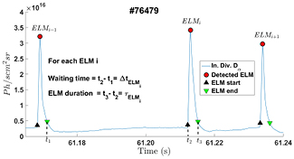
Figure 1. Illustration of the extraction of ELM waiting times ( ) and ELM durations (
 ) from a time trace of
  radiation at JET's inner divertor.
Download figure:
Standard image High-resolution image
Figure 2. Illustration of ELM energy loss (WELM) estimation from the equilibrium stored energy (WMHD), synchronized to the time trace of  radiation at JET's inner divertor.
Download figure:
Standard image High-resolution image2.3. ELM duration and slow transport events
JET ITER-like wall ELMs are sometimes followed by an extended collapse phase, called the slow transport event (STE) [22], the presence of which has been proposed to be related to divertor/scrape-off layer (SOL) conditions [23, 24] and to a change in recycling behavior in a W divertor [25, 26]. These STEs are analogous to the second phase of ELM collapse observed at ASDEX Upgrade (AUG) [24]. The typical temporal signature of an STE is shown in figures 3(a) and (b). The corresponding WELM are shown in figures 3(d)–(f).
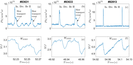
Figure 3. (a)–(c) Temporal signature of pure ELMs and ELMs followed by a slow transport event (STE) in three typical JET ILW plasmas. The N2-seeded plasmas, like CW plasmas, have narrower ELMs and no slow transport events. (d)–(f) ELM energy loss (WELM) for the pure ELMs and ELMs followed by an STE shown in (a)–(c).
Download figure:
Standard image High-resolution imageELMs accompanied by an STE have longer time scales of temperature and density collapse and result in higher total energy loss of the plasma than the losses produced by ELMs alone. We first studied the variation of the energy released by an ELM, averaged over all ELM events in a single discharge, in terms of the fraction of STEs. The latter is defined as
where  is the number of ELMs accompanied by a slow transport event and NELM is the number of ELMs that are not followed by an STE phase, hereafter referred to as pure ELMs. The ELM energy loss averaged over a single discharge, during stationary conditions, is denoted as
  and we also consider its ratio w.r.t.
  , i.e. the total stored equilibrium energy in the plasma, also averaged over the entire stationary phase of each discharge that has been investigated. The variation of
  and
and  with the fraction of STEs (fSTE) for all plasma pulses is plotted in figure 4.

Figure 4. Variation of the mean ELM energy loss ( ) and mean relative ELM energy loss (
 ) with the fraction of slow transport events (fSTE) in JET ILW plasmas.
Download figure:
Standard image High-resolution imageIn this work, we have divided JET ILW plasmas (M discharges) into three broad categories: those with a high fraction of STEs ( ), medium fraction of STEs (
 ) and those with very few or no STEs (
 ). From figure 4, a clear (linear) increase can be noticed of
  with the fraction of STEs in a plasma. A very similar conclusion is true for the relative energy loss
  , which shows that an increased energy loss is due to a higher fraction of STEs. This is in accordance with recent studies wherein it was seen that the STEs carry a significant proportion of the energy of the total ELM event [22]. STEs are absent in the JET CW database analyzed in this work. Furthermore, they disappear in N2-seeded ILW JET plasmas [22], as does the second part of the ELM collapse in AUG plasmas [24]. JET ILW ELMs, compared to JET CW plasmas have larger ELM durations (
 ). This too, in a large part, is due to the existence of STEs in ILW plasmas. The average duration
  of all ELM events during a period of stationary plasma conditions, for the plasmas analyzed in this work, are listed in table 2.
Table 2. Typical ELM durations (mean ( ) and standard deviation (std
 )) for unseeded JET ILW plasmas (varying degrees of slow transport events), N2-seeded JET ILW plasmas and JET CW plasmas.
 (ms) (ms) | std (ms) (ms) | |
|---|---|---|
| ILW | ||

| 7.1 | 3.8 |

| 3.4 | 2.2 |

| 2.7 | 0.8 |
| N2-seeded | 2.5 | 0.8 |
| CW | 2.6 | 1.2 |
N2-seeded ILW plasmas and ILW plasmas with low fSTE have  similar to CW plasmas. ILW plasmas with high fSTE exhibit
  about three times larger than the
  of CW plasmas. An investigation into the distribution of
  yields that the non-seeded JET ILW plasmas (high fSTE) have a distribution of
  which is distinctly different from N2-seeded JET ILW plasmas and JET CW plasmas. The latter two cases exhibit similar distributions for
  .
.
Figures 5(a)–(c) present the distribution of  for non-seeded JET ILW plasmas (high fSTE), N2-seeded JET ILW plasmas and JET CW plasmas. The distribution of
  for non-seeded JET ILW plasmas (high fSTE) is bimodal (two local maxima). The bimodal distribution arises as a mixture of two underlying unimodal distributions emerging from collapses due to pure ELMs and collapses followed by STEs. We performed a manual separation of pure ELM events from the cases with STEs, and the corresponding unimodal distributions are shown in figures 5(d) and (e), respectively. The pure ELMs have a duration
  that is typically less than about 5 ms, while the ELMs with STEs can last up to 14 ms. The distribution of
  for pure ELMs in high fSTE ILW plasmas (figure 5(d)) appear similar to the distribution of
  for N2-seeded JET ILW plasmas (figure 5(b)) and JET CW plasmas (figure 5(c)). These distributions are visibly non-Gaussian with a strong positive skew and we verified that a similar degree of skewness also exists in the distribution of ELM durations from individual discharges. From the physical point of view it means that, in our data set, pure ELMs with durations longer than 4–5 ms are relatively rare, compared to the prevailing duration of about 2.5 ms. From the statistical point of view, characterization of skewed distributions necessitates additional metrics such as median and mode. The means and standard deviations alongside medians, and skewness estimates for each distribution are summarized in table 3.
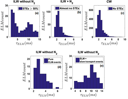
Figure 5. Distribution of ELM durations for various subsets of JET plasmas investigated in this work. In each panel, the vertical axis shows the number of ELM events. (a) Unseeded ILW plasmas with a high fSTE, (b) N2-seeded ILW plasmas, (c) CW plasmas, (d) Pure ELMs from high fSTE unseeded ILW plasmas, (e) ELMs followed by STEs from high fSTE unseeded ILW plasmas.
Download figure:
Standard image High-resolution imageTable 3. Summary (mean ( ), standard deviation (std
 ), median (
 ) and skewness) for the distributions of ELM durations extracted from the JET discharges investigated in this work.
| JET plasmas |
 (ms) (ms) | std (ms) (ms) |
 (ms) (ms) | Skewness | |
|---|---|---|---|---|---|
| ILW plasmas | Pure ELMs | 3.2 | 0.87 | 3.0 | 0.23 |

| ELMs + STEs | 9.6 | 2.5 | 9.8 | 0.08 |
| N2-seeded ILW plasmas | 2.5 | 0.81 | 2.3 | 0.25 | |
| CW plasmas | 2.6 | 1.2 | 2.3 | 0.25 | |
Here, the skewness was estimated not from the third-order moment of the distribution (which typically requires a lot of data points), but by dividing the difference between mean and median with standard deviation. For gaining an interesting insight into skewness estimation, the reader may refer to [27]. Contrary to pure ELM events, the distribution of  for ELMs followed by STEs in high fSTE JET ILW plasmas (figure 5(e)) follows a more symmetric distribution.
2.4. Tools for correlation analysis
For analyzing the relation between ELM waiting times and energy losses, as a first step we use scatter graphs to get a qualitative impression. Furthermore, in order to quantify the strength of linear relation between  and WELM for individual ELMs within single discharges, the regular Pearson's product moment correlation coefficient (ρ) is estimated. Background theory can be found in [28–31]. Herein, we present a brief simplified summary tailored to our limited needs.
For two related sets of data that can be modeled as outcomes of random variables X and Y, this correlation coefficient is defined as,
where cov stands for the covariance between the variables, while  and
and  are their standard deviations. The coefficient
  takes values in the range [−1, 1]; a value of 1 means that X and Y are perfectly linearly correlated, a value of 0 that there is no correlation, while a value of −1 that they are perfectly anti-correlated.
Further statistical inference that we will perform in various situations, based on the estimates of ρ include estimation of confidence intervals, testing the significance of correlations and regressing against a set of global engineering parameters. This is complicated by the fact that the standard estimate of ρ has a non-Gaussian distribution. Therefore estimates r of ρ are converted to a z-value, the approximate distribution of which has been well investigated for a bivariate normal parent distribution:
For reasonable sample sizes, the mean of the distribution is close to the z-value itself, while the standard deviation does not notably depend on ρ and can be approximated by  , where n is the number of data points. For non-normal parent distribution, the distribution of z is more complicated, see [31].
Further, we follow standard hypothesis test procedures [30] in testing the significance of correlation r. First, we specify the null (Ho ) and alternative (HA ) hypotheses:


Under the hypothesis  , the following test statistic t is known to follow a Student-t distribution with N − 2 degrees of freedom,
Given that the null hypothesis is true, the probability ('p-value') of obtaining a value as large as t or greater is determined. If the p-value is smaller than the pre-set significance level α, the null hypothesis is rejected and ρ is deemed to be significantly different from zero. The value of α is customarily taken as 0.05 and occasionally, especially for large sample sizes (say n between 100 and 1000), more stringently as 0.01.
In addition, we use an alternative measure of correlation, known as Spearman's rank correlation coefficient rs, which measures monotonic dependence between X and Y:
where Xi
denotes the rank of the value Xi
in the ordered series of values of the variable X. The estimate rs is a nonparametric measure of dependence and compared to r is much less sensitive to outliers. Similar to r, rs is in the interval [−1, 1] and  implies no monotonic dependence.
Finally, partial correlation is used when investigating ELMs from different plasmas. Partial correlation measures the degree of association between two random variables while correcting for the effect of another variable, or several other variables, on this relation. The partial correlation of X and Y, adjusted for Z is:
Partial correlation can also be computed for Spearman's rank correlation coefficient.
3. Analysis of the relation between ELM properties
The relation between WELM and  , averaged over all ELMs in a single discharge, is shown in figures 6(a) and (b) for ILW and CW plasmas, respectively. In agreement with the findings in [18], there is a strongly positive correlation between WELM and
  for ILW plasmas as well as for CW plasmas. Likewise, as shown in figures 6(c) and (d) there is a strong linear relationship between average relative ELM energy loss
  and
and  . However, ELM control is targeted at influencing the energy loss of individual ELMs. Thus, basing the mitigation strategy on the relation between the average properties of different plasmas can possibly be an oversimplification. Furthermore, the relation presented in [18] does not take into account the uncertainty on WELM and
  . Nevertheless, it can be observed from figure 7 that the standard deviation of WELM and
  is substantial and increases roughly linearly with the mean value. A straightforward extrapolation based on figure 7(b) would suggest 7–10 MJ of standard deviation around an absolute WELM of 20–30 MJ at ITER.
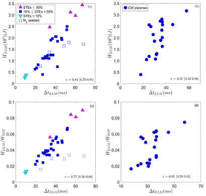
Figure 6. Scatter graphs between  and
and  for (a) JET ILW plasmas, (b) JET CW plasmas. Estimates for the Pearson correlation coefficient (r) are indicated, together with the 95% confidence interval.
Download figure:
Standard image High-resolution image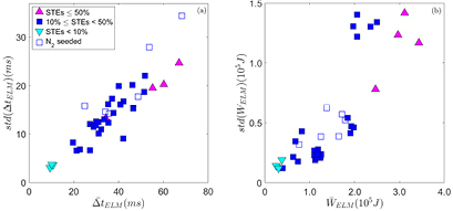
Figure 7. Scatter graphs between mean and standard deviation of (a)  and (b) WELM, for the JET ILW plasmas.
Download figure:
Standard image High-resolution imageIn general, the probability distributions of ELM properties contain comprehensive information about their variability [32–34] and therefore studying their statistical correlation properties will yield a better insight into the strength of any existing relations. Figure 8 is a reproduction of figure 6, with the addition of the error bars indicating a single standard deviation. The strongly linear relations depicted in figure 6 appear to be less clear with the inclusion of standard deviations in figure 8. Hence, as will be shown below, the effect of the spread in WELM and  within each plasma is better quantified by studying the relation between WELM and
  for individual ELMs in a discharge. Furthermore, the relation between
  and
and  for ILW and CW plasmas is shown in figures 9(a) and (b). The correlation is clearly different in the two cases: ILW plasmas exhibit a strongly positive correlation, whereas CW plasmas appear to have no correlation. Further, the correlation coefficient r for the CW plasmas does not reject the null hypothesis of zero correlation at 5% significance level. This provides a quantitative affirmation of a lack of correlation. As a next step, the correlation between
  and
and  is examined in figures 9(c) and (d). This too reveals a trend in correlation similar to that observed in figures 9(a) and (b). Next, the ILW plasmas are split into two groups and the correlation analysis is performed on each group separately. As indicated in figure 9(c), the first group comprises of plasmas with
  ms and the second group consists of plasmas with
  ms. The plasmas in the first group have
  comparable to the
  of the CW plasmas analysed in this work whereas the plasmas in the second group have a relatively high fSTE and
  greater than the
  of the analysed CW plasmas. It can be noted from figure 9(c) that each of the two groups exhibit a high correlation between
  and
and  . The high correlation exhibited by the first group of ILW plasmas indicates that strong correlation between
  and
and  cannot be fully attributed to the presence of STEs in the ILW plasmas.
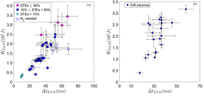
Figure 8. Scatter graphs between  and
and  , including the error bars specified by a single standard deviation, for (a) JET ILW plasmas, (b) JET CW plasmas.
Download figure:
Standard image High-resolution image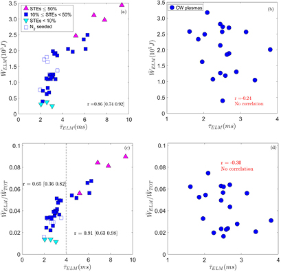
Figure 9. Scatter graphs between  and
and  for (a) JET ILW plasmas, (b) JET CW plasmas. Scatter graphs between
  and
and  for (a) JET ILW plasmas, (b) JET CW plasmas. Estimates for the Pearson correlation coefficient (r) are indicated, together with the 95% confidence interval. In (c) r values for the two groups of ILW plasmas (
 ms and
  ms) are indicated. CW plasmas, in contrast to ILW plasmas, do not reject the null hypothesis of zero correlation at 5% significance level.
Download figure:
Standard image High-resolution image3.1. Properties of individual ELMs
After studying the ELM properties averaged over a window of stationary plasma conditions, we now concentrate on relations between the properties of the individual ELMs. Estimates of the correlation between WELM and  (
( ), along with 95% confidence intervals are presented in figures 10 and 11 for individual ELMs in JET ILW and JET CW plasmas, respectively. Despite
  and
and  conforming to the expected inverse dependence between WELM and fELM, the correlation between WELM and
  for individual ELMs varies from being strongly correlated for certain plasmas to being uncorrelated for others. This is observed in both CW as well as ILW plasmas. Compared to ILW discharges, CW plasmas on the whole have higher correlation between WELM and
  for individual ELMs, with 12 out of the 20 (60%) analyzed plasmas exhibiting high correlation (r > 0.40) and 4 out of the 20 (20%) analyzed plasmas demonstrating no correlation (
 ). On the other hand, out of the 38 ILW plasmas, only the 6 (16%) N2-seeded plasmas exhibit high correlation (r > 0.40), whereas 19 (50%) plasmas show no correlation and 13 (34%) have a medium correlation.
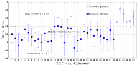
Figure 10. Estimates of linear correlation between WELM and  for individual ELMs in JET ILW plasmas. 95% confidence intervals are also indicated. Discharges indexed 33 to 38 are N2-seeded plasmas.
Download figure:
Standard image High-resolution image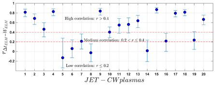
Figure 11. Estimates of linear correlation between WELM and  for individual ELMs in JET CW plasmas. 95% confidence intervals are also indicated.
Download figure:
Standard image High-resolution imageThe underlying processes causing WELM and  to exhibit varying degrees of correlation could be one or several of the following. The size of WELM is controlled by the pedestal parameters, i.e. the density and temperature inside the pedestal before the ELM crash [35, 36]. A multi-machine study performed on ASDEX, DIII-D, JT60U and JET CW has established that the relative ELM energy losses scale with the inverse of pedestal collisionality [35]. Other key parameters that have an important effect on WELM are the pedestal width [37], plasma rotation [38] and the plasma shape [39]. On the other hand,
  is a consequence of the various timescales involved in the recovery of the pedestal to its pre-ELM state following the ELM crash. The pedestal recovery time can be potentially modified by enhanced losses in the inter-ELM period, either by increased bulk radiation or by an increased level of density and magnetic fluctuations. WELM, being determined primarily by the pre-ELM pedestal plasma parameters, is likely to remain unaffected by the inter-ELM processes that can potentially modify
  . Furthermore, the peeling-ballooning model, which is a leading candidate for explaining ELM onset, fails to explain the phase of saturated gradients without ELMs [40]. In medium-sized tokamaks at low edge temperature, the bootstrap current seems to be fully developed for a relatively long time interval before an ELM crash. It is reasonable to assume that, after the pedestal has recovered, an additional increase in
  will not lead to an additional increase in WELM. Finally, figure 12 suggests that, in the case of the ILW plasmas, the correlation between WELM and
  for individual ELMs varies inversely with fSTE. Hence, the presence of the STEs appears to be at least partly responsible for the observed reduction in correlation between ELM waiting times and energies in ILW plasmas.
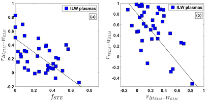
Figure 12. Variation of linear correlation between WELM and  (
( ) for individual ELMs in JET ILW plasmas. (a) With the fraction of slow transport events (fSTE) and (b) with the linear correlation between WELM and
  (
( ) for individual ELMs in JET ILW plasmas.
Download figure:
Standard image High-resolution imageFurthermore, we note that for ILW plasmas there is a weakly inverse relation between the correlation among WELM and  and the correlation among
  and WELM. It can be seen from figure 12 that plasmas with high fSTE exhibit no correlation between WELM and
  and consequently a very high correlation between
  and WELM. As an illustration, scatter plots between WELM and
  and WELM and
  for three representation plasmas are given in figure 13. On the one hand, non-seeded JET-ILW plasma #82806 with
  exhibits a very high correlation between WELM and
  and no correlation between WELM and
  . On the other hand, N2-seeded JET-ILW plasma #83179, similar to JET-CW plasma #76479, demonstrates a high correlation between WELM and
  and no correlation between WELM and
  .
.
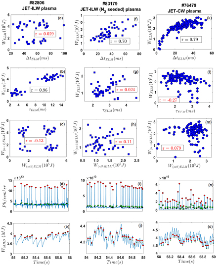
Figure 13. Scatter plot between WELM and  , WELM and
  and
and  and
and  for (a)–(c). JET pulse #82806 (unseeded JET ILW plasma (
 )), (f)–(h). #83179 (N2-seeded JET ILW plasma) and (k)–(m). #76479 (JET CW plasma). Estimates of r for each scatter plot are also specified. r estimates that do not reject the hypothesis of no correlation at 5% significance level are indicated in color red. Also given are time traces of Be II radiation from the inner divertor (ILW plasmas),
  from the inner divertor (CW plasma) and the equilibrium stored energy (WMHD).
Download figure:
Standard image High-resolution image3.2. Collective properties of individual ELMs in all analyzed plasmas
Next, the collective properties of all ELM events in our JET ILW database are investigated. A scatter diagram between WELM and  for all ELMs (excluding N2-seeded plasmas) is shown in figure 14(a). Table 4 lists the estimates for r and rs corresponding to the scatter diagram presented in figure 14(a). Partial correlations between WELM and
  , while controlling for Bt, Ip, Pinput, ne,
  and
and  , are presented as well. In this case partial correlation is a more realistic measure for assessing the relation between WELM and
  , since it takes into account the widely varying global plasma conditions across the data set. It is noteworthy that adjusting for the varied plasma conditions brings a significant reduction in the correlation. Moreover, values of rs are comparable with r, which confirms the robustness of r estimates.
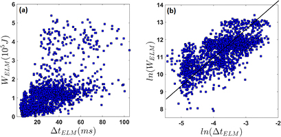
Figure 14. Scatter graph between (a) WELM and  , (b) Logarithm of WELM and
  for all ELMs in JET ILW plasmas. The least-squares line of best fit to the logarithm of WELM and
  is also shown.
Download figure:
Standard image High-resolution imageTable 4. Estimates of regular and partial correlations, based on Pearson (r) and Spearman (rs) coefficients, between WELM and  for all ELMs in the JET ILW plasmas. The partial correlations control for Bt, Ip, Pinput, ne,
  and
and  .
.
| r | rs | |
|---|---|---|
| Regular | 0.58 | 0.65 |
| Partial | 0.21 | 0.26 |
Furthermore, in order to account for any variation of the standard deviation of the data (heteroscedasticity), which is especially clear in figure 14(a) (see also figure 7), a scatter diagram between the logarithm of WELM and  for all ELMs in the analyzed ILW plasmas (excluding N2-seeded plasmas) is shown in figure 14(b). Also, on figure 14(b), the least-squares line of best fit is indicated and the corresponding regression coefficients are given in table 5. The observed linearity in the log–log space is indicative of a power law relation between WELM and
  . This implies that the rate of change of WELM and
  decreases gradually up to a point beyond which the two quantities become almost independent. This is reaffirmed by the inspection of figure 14(a) where there appears to be a saturation of WELM for
  greater than 25–30 ms. This is also in agreement with an earlier observation of statistical independence between WELM with
  beyond
  ms, made by Webster et al [19] for individual ELMs from a set of 2 T, 2 MA JET ILW plasmas. The point beyond which WELM becomes independent of
  is likely to be limited by the pedestal recovery time and the total energy stored in the plasma. In the plasmas considered in this work, although the plasma thermal energy for pure ELMs appears to increase until the next ELM, it is largely recovered to its pre-ELM value in
  ms. This suggests a scenario in which the edge pedestal is largely restored in ≈25 ms, leading to a significant reduction in the correlation between WELM for
  beyond
  ms. On the other hand, for ELMs followed by STEs, the plasma thermal energy recovers to its pre-ELM + STE value in
  ms.
ms.
Table 5. Estimated coefficients and standard errors for the least-squares line of best fit shown in figure 14(b). The model is  .
.

|

|

|

|
|---|---|---|---|
| 14.7 | 0.895 | 0.071 | 0.019 |
Furthermore, it can be estimated that for ILW ELMs a reduction of  from 25–30 ms (beyond which WELM and
  are very weakly correlated) to 10 ms reduces WELM by ≈
 . On the other hand, a reduction of
  from 50–60 ms to 25–30 ms, reduces WELM by ≈
 . This suggests that if ELMs are consistently paced at 10 ms, WELM can be reduced by ≈60–70%.
4. Global dependence of correlation between ELM energy losses and waiting times
Since the success of ELM mitigation depends considerably on a high correlation between WELM and  , we now aim to locate the regions of plasma operational space where the corresponding correlation coefficient
  is large. One approach for studying the dependence of
  on plasma parameters would be to rely on single parameter scans. In the case of the present work, there are not enough dedicated experiments available to allow such a study. Nevertheless, as a preliminary step, in figures 15 and 16 scatter plots between the plasma engineering parameters Bt, Ip, Pinput, ne,
  ,
,  and the correlation coefficient
  are provided. It can be observed that individually none of the plasma engineering parameters discriminate well between plasmas with a high, medium or zero
  . As a next step, regression analysis is used for quantifying the effect of plasma parameters on
  . As discussed in section 2.4, the sampling distribution of r is not normal, therefore r is transformed to the quantity z in (5). Standard multilinear regression using least squares is then performed for yielding the regression coefficients given in table 6. Standard error (SE) of the regression coefficients is also given in table 6.
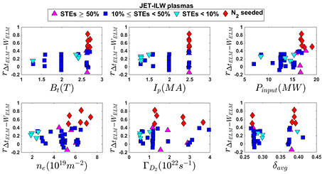
Figure 15. Scatter plots of correlation between WELM and  (
( ) and plasma engineering parameters Bt, Ip, Pinput, ne,
  and
and  for JET ILW plasmas.
Download figure:
Standard image High-resolution image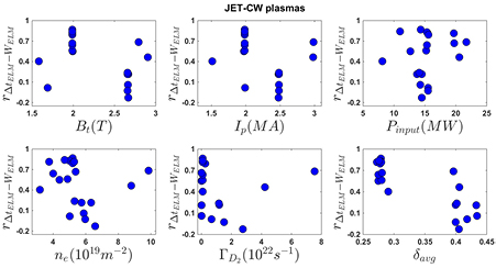
Figure 16. Scatter plots of correlation between WELM and  (
( ) and plasma engineering parameters Bt, Ip, Pinput, ne,
  and
and  for JET CW plasmas.
Download figure:
Standard image High-resolution image
Table 6. Least-squares multilinear regression fits (including a cut-off term C) for correlation between WELM and  using global plasma parameters as predictors. The coefficient estimate alongside 95% confidence intervals are presented, together with the root-mean-square error (RMSE) and the coefficient of determination (R2).
| ILW | ||||||
|---|---|---|---|---|---|---|
| CW | Model 1 | Model 2 | ||||
| Coeff | SE | Coeff | SE | Coeff | SE | |
| C | 1.67 | 0.58 | −0.457 | 0.30 | 0.0287 | 0.29 |
| Bt (T) | −0.982 | 0.64 | 0.0483 | 0.17 | 0.162 | 0.15 |
| Ip (MA) | 1.62 | 1.06 | 0.559 | 0.48 | 0.0791 | 0.38 |
| Pinput (MW) | −0.0229 | 0.031 | 0.0119 | 0.024 | 0.0080 | 0.022 |

| 0.165 | 0.13 | −0.0259 | 0.10 | −0.0486 | 0.099 |

| −0.113 | 0.070 | −0.114 | 0.075 | −0.0422 | 0.062 |

| −8.54 | 1.5 | −0.313 | 0.90 | −0.618 | 0.85 |
| fSTE | — | −1.19 | 0.27 | — | ||

| — | — | 0.269 | 0.053 | ||
| RMSE(%) | 23.4 | 18.3 | 17.4 | |||
| R2 | 0.83 | 0.64 | 0.67 | |||
The regression model for CW plasmas is constructed using Bt, Ip, Pinput, ne,  and
and  as predictor variables. For ILW plasmas, however, fSTE is included as an additional predictor variable, as it has been shown in section 3.1 that fSTE has an appreciable influence on
  . In addition, since fSTE is not strictly an engineering quantity, a second model (model 2) for ILW plasmas is constructed using
  as an additional parameter in place of fSTE. The quality of the fitted regression model is quantified with the root-mean-square error (RMSE(%)), which is an indicator of the deviation of the measurements from the model, and the coefficient of determination (
![${{R}^{2}}\in [0,1]$](https://content.cld.iop.org/journals/0029-5515/57/3/036026/revision2/nfaa5098ieqn214.gif) ), which measures the degree to which the predictor variables and the regression model explain the observed variation of the response variable. Based on the values of RMSE and R2, each model is fairly appropriate to describe the variation of the correlation.
), which measures the degree to which the predictor variables and the regression model explain the observed variation of the response variable. Based on the values of RMSE and R2, each model is fairly appropriate to describe the variation of the correlation.
It is noteworthy that a direct comparison between the regression coefficients of different parameters cannot be made as they are measured on different scales. However, an examination of the standard errors of the coefficients indicate the parameters that contribute most to the regression model. Across both model 1 and model 2 that are constructed for ILW plasmas, fSTE or alternatively  appear to be the most important determinant of
  as their coefficient estimates are much greater than the SEs. This is expected since it has earlier been noted in section 3.1 that it is only with N2 seeding that high values of
  comparable with CW plasmas are obtained. In unseeded ILW plasmas the correlation fluctuates at most to a weakly positive correlation from a state of no correlation. Secondary to
  ,
,  emerges as the more important determinant of
  . This is consistent with the model for CW plasmas as therein
  followed by
  appear to be the most important of the considered plasma engineering parameters. For the remaining parameters it can be noted that SE is comparable and sometimes slightly higher than the coefficient estimate which suggests that they are less contributory to the regression model.
It is important to note that in addition to the global time-averaged plasma engineering parameters, the regression models could substantially benefit if the complete distributions of the predictor parameters would be considered.
5. Relation between energy loss of successive ELMs
Finally, the relationship between energy losses of consecutive ELMs is investigated. As can be noted from table 7, only 10–15% of the analyzed JET-ILW (including N2-seeded plasmas) and JET-CW plasmas exhibit a weak non-zero correlation. Also, the values of rs are in agreement with estimates of r. WELM of consecutive ELMs is largely uncorrelated. This implies that an ELM with a large WELM is equally likely to be followed by an ELM with a large or small WELM. Further, this observation is consistent across unseeded JET-ILW plasmas, N2-seeded JET-ILW plasmas and JET-CW plasmas. This can also be observed in the scatter plots of WELM of nth ELM and WELM of (n + 1)th ELM in figure 13. For each of the three representative plasmas, #82806, #83179 and #76479, WELM of successive ELMs is uncorrelated.
Table 7. Number of ILW plasmas (including N2-seeded plasmas) and CW plasmas with correlation between energy loss of successive ELMs r > 0.3,  and
and  . The number of plasmas with r significantly different from zero are also indicated at two significance levels α.
| Plasmas |

|

| r > 0.3 |


|


|
|---|---|---|---|---|---|
| ILW | 20 | 15 | 3 | 4 | 2 |
| CW | 16 | 4 | 0 | 3 | 0 |
6. Conclusions
This work examines the relation between WELM and  for individual ELMs in a set of non-seeded JET-ILW plasmas and compares the results with a set of N2-seeded JET-ILW plasmas and JET-CW plasmas. It is found that the empirically established inverse relation between average fELM and
  is not ubiquitously obeyed by individual ELMs. The linear correlation between WELM and
  varies from being strongly correlated for certain plasmas to being completely uncorrelated for others. CW plasmas, in general, exhibit higher correlation between WELM and
  than ILW plasmas and it is only in N2-seeded ILW plasmas that a high correlation comparable to certain CW plasmas is observed.
Furthermore, ELMs in non-seeded JET ILW plasmas are often followed by a slow transport event resulting in a bi-modal distribution of ELM durations. The two modes correspond to two distinct underlying phenomena: pure ELMs and ELMs followed by a slow transport event. Slow transport events are not present in JET-CW plasmas and they disappear in N2-seeded JET-ILW plasmas, giving rise to a unimodal asymmetric distribution of ELM durations. The average ELM energy loss in a plasma scales linearly with the proportion of ELMs followed by slow transport events in a plasma, whereas the linear correlation between WELM and  varies inversely with the fraction of slow transport events.
A collective analysis of all the ELMs from the unseeded JET-ILW ELMs plasmas revealed that the variation between WELM and  obeys a power law relationship. WELM appears to saturate for
  –30 ms which is roughly the time taken for the plasma thermal energy to return to its pre-ELM value. This suggests a scenario where the linear correlation between WELM and
  significantly reduces as the edge pedestal recovers to its pre-ELM value.
Moreover, least squares linear regression has been employed for determining the region of the plasma operating regime where the correlation between WELM and  is maximized. A regression model is constructed using plasma and engineering parameters for both JET-ILW and JET-CW plasmas. While the models will certainly benefit from more informative predictors, they nevertheless indicate the more important parameters from the plasma parameters used as predictors. For the JET-ILW plasmas,
  followed by
  and
and  contribute most to the correlation between WELM and
  . Similarly, for JET-CW plasmas
  and
and  appear to be the most important determinants of correlation.
Lastly it is acknowledged that WELM and  are stochastic quantities and a precise analysis of these quantities needs to effectively incorporate the uncertainty on these quantities. It has also been shown that the standard deviation of WELM and
  increases linearly with the mean value. Analyzing WELM and
  for individual ELMs subtly allows for the standard deviation in WELM and
  to be accommodated and indeed reveals additional information. It is emphasized that analyzing complete probability distributions of WELM,
  ,
,  and other plasma parameters will yield a more comprehensive picture and will thus form the basis of future investigations.
Acknowledgment
This work has been carried out within the framework of the EUROfusion Consortium and has received funding from the EURATOM research and training programme 2014–2018 under grant agreement No 633053. The views and opinions expressed herein do not necessarily reflect those of the European Commission. The authors would like to thank Dr. Lorenzo Frassinetti for his useful feedback on this work.
Footnotes
- 4
We here mention also recent work concerning the multi-machine scaling of ELM heat loads deposited at the divertor (Eich PSI 2016).