


Abstract
A new model for the edge harmonic oscillations (EHOs) in the quiescent H-mode regime has been developed, which successfully reproduces the recent observations in the DIII-D tokamak. In particular, at high E × B flow shear only a few low-n kink modes remain unstable at the plasma edge, consistent with the EHO behavior, while at low E × B flow shear, the unstable mode spectrum is significantly broadened, consistent with the low-n broadband electromagnetic turbulence behavior. The model is based on a new mechanism for destabilizing low-n kink/peeling modes by the E × B flow shear, which underlies the EHOs, separately from the previously found Kelvin–Helmholtz drive. We find that the differential advection of mode vorticity by sheared E × B flows modifies the 2D pattern of mode electrostatic potential perpendicular to the magnetic field lines, which in turn causes a radial expansion of the mode structure, an increase of field line bending away from the mode rational surface, and a reduction of inertial stabilization. This enhances the kink drive as the parallel wavenumber increases significantly away from the rational surface at the plasma edge where the magnetic shear is also strong. This destabilization is also shown to be independent of the sign of the flow shear, as observed experimentally, and has not been taken into account in previous pedestal linear stability analyses. Verification of the veracity of this EHO mechanism will require analysis of the nonlinear evolution of low-n kink/peeling modes so destabilized in the linear regime.
Export citation and abstract BibTeX RIS
1. Introduction
How E × B flow shear influences plasma instability is a long-standing issue in the field of plasma physics. The E × B flow shear was considered responsible for the suppression of plasma edge turbulence [1], leading to a spontaneous transition from a low confinement state (L-mode) to a high confinement state (H-mode) in tokamaks [2]. The instabilities behind the edge plasma turbulence are small in scale (high-n, n is the toroidal mode number) [3]. For large-scale (low-n) magnetohydrodynamics (MHD) instabilities, such as kink/peeling modes [4], whether and how the E × B flow shear can significantly modify these stabilities is still an open question.
The kink/peeling mode is believed to be the dominant instability triggering large edge-localized modes (ELMs) at low collisionality in the H-mode plasma edge, a region so-called 'pedestal' where steep density and temperature gradients develop [4]. Large ELMs are a serious concern for next-generation fusion devices because of the intolerable high transient heat loads that they can impose on the plasma-facing wall materials [5]. However, the particle transport driven by ELMs can help prevent impurity accumulation and sustain plasma performance. A robust control of ELMs while retaining good thermal confinement and sufficient edge particle transport for impurity exhaust is therefore essential for fusion energy production.
One potential solution for large ELMs is the quiescent H-mode (QH-mode) regime [6–8], in which ELMs are replaced by the edge harmonic oscillations (EHOs). EHOs play an important role in avoiding ELMs and sustaining stationary operations with good thermal confinement and sufficient particle transport for impurity removal. The thermal confinement improvement factor, H98,y2, associated with the QH-mode is typically comparable or even higher than that in the type-I ELMy H-mode, and the impurity confinement time in the QH-mode is comparable to that in the type-I ELMy H-mode, suggesting that EHOs may exhaust impurities as effectively as large ELMs. Recent experiments and theories suggested [4, 9] that the EHOs might have been saturated low-n kink/peeling modes partially destabilized by the E × B flow shear. The EHO saturation was thought due to relaxation of the rotation shear by a braking effect induced by EHO-driven momentum transport [4, 10] rather than growing explosively like an ELM. Understanding the physics of EHOs is required in extending the QH-mode operation regime to future fusion reactors.
QH-mode is usually obtained with strong toroidal rotation shear at the plasma edge [6–8]. The EHO is thought to be partially driven by the E × B flow shear, as supported by a couple of observations. For example, QH-mode favors counter-Ip plasma rotation [8], which reinforces the diamagnetic rotation in determining the Er from radial force balance. Indeed, QH-mode plasmas are found to have a significantly deeper negative Er well than in the ordinary ELMy H-mode plasmas [6–8]. A more careful analysis of the Er profile in QH-mode plasmas suggests that it is more likely the Er shear determines the QH-mode access, rather than the impurity carbon ion toroidal rotation [11]. This conclusion was further confirmed in observations where the QH-mode is sustained at nearly zero neutral beam injection (NBI) torque and toroidal rotation, and a strong edge E × B shear is sustained by the counter-Ip torque injection from the applied non-axisymmetric non-resonant magnetic fields [11, 12].
Very recently, a new QH-mode regime was observed in the DIII-D tokamak at low rotation [13], where a low-n broadband electromagnetic turbulence replaced the coherent EHOs in the pedestal region. Here, a reduced E × B flow shear in the edge pedestal was linked to this change of edge mode behaviors. Low rotation and rotation shear are anticipated in the pedestal region of future fusion plasmas, since the plasma moment of inertia is much larger than that in today's devices, and the applied torque is limited. The QH-mode access under this condition therefore becomes important.
The effects of E × B flow shear on the peeling/ballooning mode stability have been studied numerically. Early pedestal stability analysis with single-fluid ideal-MHD codes ELITE [4] and MINERVA [14] showed that the toroidal rotational shear is stabilizing for high-n modes and destabilizing for low-n modes. The stabilization of high-n modes by toroidal rotational shear has been used to explain ELM mitigation by rotation in experiments. For example, significant reduction of ELM size and increase of ELM frequency was observed in the JT-60U tokamak with increased toroidal rotation in the direction counter to the plasma current (counter-Ip) and more negative radial electric field, Er, at the plasma edge [15]. However, the destabilization of low-n modes was estimated to be relatively small (a few percent or less in growth rate) [4].
Destabilization of the low-n modes was seen in recent MHD simulation using M3D-C1 [16] and BOUT++ [17] codes. A linear eigenmode analysis of the EHO-like low-n modes using M3D-C1 indicated that these modes were destabilized by rotation and/or rotation shear, independently of the rotation direction [16]. This is consistent with the earlier observations of EHOs [8] and supports the view that the EHOs are saturated low-n kink/peeling modes destabilized by edge E × B flow shear [4, 9]. However, the underlying mechanisms for destabilization and the associated mode growth rates were not identified.
Simulation study with a two-fluid reduced MHD code BOUT++ suggested that the E × B flow shear destabilizes peeling-ballooning modes mainly through the Kelvin–Helmholtz (K–H) drive [17]. Previously, the K–H instability was shown to be stabilized in the tokamak plasma edge by strong magnetic shear [18]. However, a most recent BOUT++ simulation [19] indicated that the mode remained unstable even after the K–H drive was turned off artificially. These developments therefore beg the question: how could the E × B flow shear destabilize the kink/peeling mode in the absence of the K–H drive?
To address this issue, the effects of E × B flow shear on the linear stability of the low-n kink/peeling mode are studied in detail via a linear eigenvalue analysis guided DIII-D experimental data. We discover that the E × B flow shear can destabilize the low-n kink/peeling mode through a new mechanism, separately from the K–H drive [17]. Our analysis indicates that the differential advection of mode vorticity by sheared E × B flows modifies the 2D pattern of mode electrostatic potential perpendicular to the magnetic field lines, which in turn causes a radial expansion of the mode structures, an increase of field line bending away from the mode rational surface, and a reduction of inertial stabilization. These in turn enhance the kink drive as the parallel wavenumber increases significantly away from the rational surface where the magnetic shear is also strong. This enhanced destabilization by E × B flow shear may well be the underlying mechanism for the generation of EHOs and/or low-n broadband electromagnetic turbulence in the QH-mode pedestal. Our results reproduce the observations that at high E × B flow shear only a few low-n modes remain unstable, consistent with the EHO behavior, while at low E × B flow shear the mode spectrum is significantly broadened, consistent with the low-n broadband electromagnetic turbulence behavior observed recently in the DIII-D tokamak. Furthermore, this destabilization is shown to be independent of the sign of the flow shear, consistent with the experimental observations of EHO in the QH-mode plasmas at both negative and positive rotations [8].
On the other hand, the kink/peeling mode is considered the dominant instability leading to large ELMs at low collisionality, a condition anticipated in the pedestal region of future fusion plasmas [4]. Moreover, low rotation and rotation shear are very likely an essential feature of future fusion plasmas. The E × B flow shear in the pedestal region could therefore be much smaller than that with high-torque injection in today's devices, as indicated in the recent DIII-D experiments [13]. Our results suggest that the kink/peeling instability is strongly dependent on the E × B flow shear at the plasma edge. ELM behaviors in future low-rotation fusion plasmas can therefore be very different from those in today's devices where strong torque injection and strong E × B flow shear prevail at the plasma edge. The required active control and mitigation of the ELMs could therefore be different.
Furthermore, our findings point to a possible mechanism of ELM control via the resonant magnetic perturbations (RMPs). Significant Er profile change at the plasma edge usually accompanies the application of RMPs [20–26]. Our results suggest that the E × B flow shear may influence ELMs through its influence on the kink/peeling instabilities. Whether the RMP prevents ELMs by inducing Er profile change is therefore of high interest.
In the next section, a schematic 2-dimentional (2D) fluid model is used to illustrate how E × B flow shear induces radial expansion of mode electrostatic potential structure. In the third section, the radial expansion effect is studied analytically. In the fourth section, we propose a new model of kink/peeling mode in the helical coordinate system [3], derive the linear eigenvalue equation, and calculate dispersion relation using the energy principle. In the fifth section, we conduct a linear eigenvalue analysis of a typical QH-mode discharge measured in DIII-D [13]. Finally, discussions and a summary are presented in the last section.
2. Illustration of the new physics using a schematic 2D fluid model
In this section, a highly simplified 2D fluid model is used to illustrate the effect of E × B flow shear induced radial expansion of mode electrostatic potential structures. The model is written in the slab geometry with coordinates  , satisfying the right hand relation,
  , where e is the unit vector, y is the poloidal coordinate,
  is the radial coordinate and
  is the radial location of a rational magnetic surface. There is a uniform magnetic field B along the z axis and a background equilibrium sheared E × B flow,
  , in the y direction driven by the equilibrium radial electric field,
  , where
  is the stationary electrostatic potential. The electron diamagnetic direction is the positive direction of y. In addition, there is an ion-pressure gradient,
  , pointing radially inward, i.e. negative in x, and an E × B flow shear with a constant shearing rate,
  , in the x direction, i.e. the velocity difference,
  , is a linear function of x, where
  is the equilibrium poloidal E × B flow velocity on the rational surface.
The simulation domain is a square 2D area,  , with a periodic boundary condition and one wavelength of the dominant Fourier mode in the y direction. Thus, the poloidal wavenumber is
  . The rational surface is placed at the center of the x domain, i.e.
  . The Dirichlet boundary condition is applied to the x direction and all fluctuation quantities are fixed at zero on the x boundaries. The simulation domain consists of 99 230 triangular elements with a maximum element size of 2 mm which is smaller than the ion sound Larmor radius,
  , in the simulation, where,
  is the ion sound speed,
  is the ion gyro-frequency,
  is the mass for deuterium ions,
  is the electron temperature on the rational surface and
  .
.
The model is composed of two coupled equations.


Equations (1) and (2) are the linearized vorticity equation and ion-pressure equation, respectively. We have separated the fluctuation quantities and equilibrium quantities as usually done in fluid simulations [27], e.g. the generalized vorticity  , the ion pressure
  and the electrostatic potential
  . The generalized vorticity is also known as 'polarization charge' [28].
The fluctuating generalized vorticity is defined by 

 [27], where
  is the ion density, which is assumed to be a constant in the simulation domain for simplicity,
  ,
,  is the unit vector along the background equilibrium magnetic field,
  is the leading order perpendicular ion flow velocity,
  is the effective electrostatic potential fluctuation and
  is the ion charge state. Here,
  for singly charged ions. The electrostatic potential fluctuation,
  , is solved numerically from the Poisson's equation,
  .
.
The equilibrium generalized vorticity is defined by 
 [17], where
  is the equilibrium perpendicular ion flow velocity,
 is the equilibrium effective electrostatic potential and
  is the parallel equilibrium current density. Here, positive
  is in the electron diamagnetic direction. The field line curvature is zero in this model,
  . The
. The  term of
  is usually very small in a tokamak. In this model, the equilibrium parameters are selected to ensure
  in the simulation domain, so that the K–H drive term,
  [17], does not appear in the vorticity equation, equation (1). We avoid involving the K–H drive, since the purpose of this paper is not to study the effects of K–H drive.
The amplitude of generalized vorticity fluctuation,  , grows exponentially in this model, driven by a linear term on the right-hand side of equation (1) with a constant growth rate
  . In the meantime,
  is advected by an equilibrium sheared E × B flow in the poloidal direction, which distorts the vorticity structures, as shown in the first-row plots of figures 3 and 4. We use the velocity difference,
  , as the advection velocity, implying that the simulation box is moving with the mode structure and the mode on the rational surface is at rest in the reference frame of the simulation box.
The ion-pressure fluctuation,  , is driven by the radial E × B convection,
  , of the background equilibrium ion-pressure gradient and damped by a diffusion term on the right-hand side of equation (2) with a ion thermal conductivity,
  . In order to ensure the numerical stability, a hyper ion thermal conductivity of
  is used, which is much larger than the typical value,
  , in the tokamak edge plasma. However, this damping term does not influence the growth of
  , since the equation (1) has been designed to avoid coupling
  into equation (1), so that the time evolution of
  is independent of
  or
or  . This is similar to the situation of the MHD modes, like the kink mode, where the instability is mainly driven by the equilibrium current-density gradient, rather than the equilibrium ion-pressure gradient directly.
In order to study the effect of E × B flow shear on the mode electrostatic potential structures, we change the E × B shearing rate,  , and the ion-pressure gradient,
  , to examine five cases with different equilibrium profiles, as shown in figure 1. Note that some of the panels in figure 1 do not have 5 curves, since some curves overlap. Case 1: zero shear,
  . Case 2: negative shear with shearing rate
  . Case 3: negative shear with shearing rate
  . Case 4: positive shear with shearing rate
  . Case 5: positive shear with shearing rate
  and zero ion-pressure gradient on the rational surface,
  . For Cases 1–4, the ion-pressure gradient is the same on the rational surface,
 with
with  the right end of the x domain, as shown in figure 1(d). The ion diamagnetic frequency on the rational surface is
  .
.
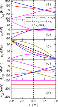
Figure 1. Background equilibrium parameter profiles in the schematic 2D fluid model for five cases with different E × B shearing rate  and ion-pressure gradient
  , as indicated by curves in different colors. (a) Sheared E × B flow
  , (b) electrostatic potential
  , (c) ion pressure
  , (d) ion-pressure gradient
  , (e) poloidal ion flow velocity
  .
.
Download figure:
Standard image High-resolution imageThe equilibrium electrostatic-potential profile, as shown in figure 1(b), is designed as 
 with
with  on the rational surface and
  on the right end, which determines the value of
  . The equilibrium ion-pressure profile,
 ![${{p}_{\text{i0}}}={{p}_{\text{i0right}}}+e{{n}_{\text{i0}}}\left[{{\varphi}_{\text{0right}}}-{{\varphi}_{0}}+B{{v}_{\text{i}y0}}\left(x-{{x}_{\text{right}}}\right)\right]$](https://content.cld.iop.org/journals/0029-5515/57/8/086047/revision2/nfaa7975ieqn095.gif) with
with  on the right end, as shown in figure 1(c), is designed to ensure the equilibrium generalized vorticity equal to zero in the simulation domain,
  . For Case 3 with
  , we set the ion-pressure gradient on the right end equal to zero,
 ![${{\left({{\partial}_{x}}{{p}_{\text{i}0}}\right)}_{\text{right}}}=e{{n}_{\text{i}0}}B\left[{{v}_{\text{i}y0}}-\left({{v}_{Ey0\text{s}}}+{{S}_{v}}{{x}_{\text{right}}}\right)\right]=0$](https://content.cld.iop.org/journals/0029-5515/57/8/086047/revision2/nfaa7975ieqn099.gif) , which guarantees no negative ion pressure in the simulation domain. This determines the value of
, which guarantees no negative ion pressure in the simulation domain. This determines the value of  in Case 3. Since
  has been fixed,
  changes with
  case by case, as shown in figure 1(e).
The initial conditions of the simulation is  and
and  with only one dominant Fourier mode at poloidal wavenumber
  , where
  is the radial amplitude profile, which is a Gaussian distribution centering at the rational surface with a radial decay length of
  . The initial peak amplitude is set at
  .
.
Figure 2 shows the time evolution of the peak value of the normalized electrostatic potential fluctuation,  , in 4 µs of linear growth. It grows exponentially with time. By fitting the curves, we obtain the effective linear growth rate,
  , of the electrostatic potential fluctuation. As indicated in figure 2,
  increases with increasing E × B flow shear and is independent of the sign of the shearing rate or the ion-pressure gradient. It exhibits the same growth rate even with flat ion-pressure gradient, which clearly demonstrates that the effect is induced by E × B flow shear, not by the ion-pressure gradient. The model has been specifically designed to avoid the influence or disturbance from other factors such as the ion-pressure gradient, so that the unique effect of E × B flow shear on the mode electrostatic potential structures can be clearly isolated and identified.

Figure 2. Time evolution of the peak value of the normalized electrostatic potential fluctuation,  , in 4 µs of linear growth in the schematic 2D fluid model for five cases with different E × B shearing rate
  and ion-pressure gradient
  , as indicated by scatters in different colors. The curves in the same colors are their exponential fit.
Download figure:
Standard image High-resolution imageThe effective linear growth rate,  , increases by ~30% from zero shearing rate to a shearing rate of
  . This increase is due to a radial expansion of the mode electrostatic potential structures away from the rational surface, which increases the radial scale length,
  , and thus reduces the effective perpendicular wavenumber,
  , of the structures, as illustrated by the simulation in figures 3 and 4. Since the linear growth rate of the generalized vorticity fluctuation,
  , is fixed at
  by the model. The reduction of
  leads to an increase in the amplitude of the mode electrostatic potential fluctuation,
  , and a reduction in the radial curvature of the mode electrostatic potential structures,
  , thus reduces the inertial stabilization associated with the mode and increases the effective linear growth rate of
  .
.

Figure 3. Snap shots of the 2D distributions of the fluctuating generalized vorticity  (first row), the fluctuating electrostatic potential
  (second row) and the fluctuating ion pressure
  (last row) at 2 µs during mode linear growth in the schematic 2D fluid model for five cases with different E × B shearing rate
  and ion-pressure gradient
  .
.
Download figure:
Standard image High-resolution image
Figure 4. Snap shots of the 2D distributions of the fluctuating generalized vorticity  (first row), the fluctuating electrostatic potential
  (second row) and the fluctuating ion pressure
  (last row) at 4 µs during mode linear growth in the schematic 2D fluid model for five cases with different E × B shearing rate
  and ion-pressure gradient
  .
.
Download figure:
Standard image High-resolution imageLet us look into the simulation results in more detail. Figures 3 and 4 shows  (first row),
  (second row) and
  (last row) in the five cases at 2 µs and 4 µs during mode linear growth, respectively. We have the following observations. With increasing shearing rate
  from 0 to
  , the mode electrostatic potential structures expand radially away from the rational surface. This radial expansion is independent of the selection of the diffusion coefficient
  in the ion-pressure equation, equation (2). The radial expansion increases with time from 2 µs to 4 µs. There is no radial expansion when the flow shear is absent, for Case 1,
  , even the ion-pressure structures are broader than the mode electrostatic potential structures. The radial expansion occurs even without the ion-pressure gradient,
  , as indicated in Case 5, which indicates that the radial expansion does not need the ion-pressure gradient and is solely induced by the E × B flow shear. The generalized vorticity structures do not expand, since it is designedly driven by a constant linear growth rate,
  , and independent of
  or
or  , so that we can pin down the origin of the radial expansion.
This radial expansion effect induced by the E × B flow shear will have significant influence on the linear growth of kink mode. As coupling to the shear Alfvén wave associated with field line bending, the kink drive,  [28], is proportional to the parallel magnetic vector potential fluctuation,
  [28], which is further proportional to the mode electrostatic potential fluctuation,
  , and the effective parallel wavenumber,
  [28]. Here,
  is the mode frequency in the plasma-moving frame of reference. In ideal-MHD plasmas, the field lines are frozen in the fluid element, thus the radial expansion of the mode electrostatic potential structures will lead to field line bending radially,
  , significantly away from the rational surface driven by radial E × B convective motion. In a background magnetic field with strong magnetic shear, the angle between the helical mode structures and the helical background field lines increase as the mode structures extend radially away from the rational surface, i.e. the effective parallel wavenumber,
  , increases with x. Here,
  is the magnetic shear length and
  is the magnetic shear parameter, which are measures of the strength of the magnetic shear,
  is the safety factor and
  is the plasma major radius on the magnetic axis. Moreover, because of the field line bending, the equilibrium current-density gradient has a projection along the magnetic field lines,
  , which gives rise to the kink drive at radial locations significantly away from the rational surface, thus enhances the kink drive. Therefore, a radial expansion of the mode electrostatic potential structures increases the effective linear growth rate of the kink mode.
The radial expansion appears to be radially asymmetric about the rational surface. It expands more inwards (towards negative x) with negative shear,  , but more outwards (towards positive x) with positive shear,
  , as shown in figures 3 and 4. The ion-pressure structures also exhibit the same radial asymmetry. The radial asymmetry disappears with flat ion-pressure gradient, as indicated in Case 5, demonstrating that the radial asymmetry originates from the ion-pressure gradient. With increasing diffusion coefficient
  in the ion-pressure equation, equation (2), the radial asymmetry is reduced, because the fluctuation amplitude of
  is reduced and the spatial gradients in the structures are smoothed, which reduces the contribution of
  in the fluctuating generalized vorticity,
  .
.
Another very interesting observation is about the tilting direction of the structures. The generalized vorticity structures are tilted in the same direction as the flow shear. It reverses direction as the sign of the shearing rate,  , changes. However, the mode electrostatic potential and ion-pressure structures appear to be tilted in the opposite direction of the flow shear. It is because that the radial expansion of the mode electrostatic potential structures preferentially arises from the locations where the generalized vorticity amplitude,
  , is minimum, i.e. the radial curvature of effective electrostatic potential is minimum, as shown in figures 3 and 4. The ion-pressure structures are determined by the radial E × B convection,
  , therefore follow the tilting direction of the mode electrostatic potential structures. Although the initial tilting angle is in the opposite direction with respect to the flow shear. Comparing 2 µs with 4 µs, we find that the tilting angle changes with time and the change is still in the same direction as the flow shear.
Finally, we clarify the fundamental mechanism for the radial expansion of mode electrostatic potential structures. The central reason is that the quantity advected by the equilibrium sheared E × B flows is the polarization charge,  , not the fluctuating electrostatic potential,
  . The sheared flows advect the polarization charge poloidally, introducing a time-varying radial phase shift, which in turn modifies the radial distributions of polarization charge and thereby the radial curvature profiles of the mode electrostatic potential structures, finally leading to the radial expansion.
The detailed physical picture is as follows. For a radially localized mode electrostatic potential structure, the radial curvature,  , peaks near the rational surface and the low curvature regions are in between the positive and negative potential eddies when there is no flow shear, as shown in figures 3 and 4. The sheared flows poloidally advect the low curvature regions adjacent to the rational surface. When the low curvature regions move to the poloidal locations radially aligned with the high curvature peaks on the rational surface, the mode electrostatic potential will expand radially through those locations simply due to low curvature.
On a longer timescale during mode growth,  , the radial expansion would appear periodically with a frequency of
  , when the mode structure shifts beyond a half-wavelength poloidally, where
  is the shear frequency. However, this is prevented in our case, since the linear growth rates of MHD instabilities, such as the kink/peeling modes, are usually much larger than the shear frequency,
  , so that the growth time is too short to allow the structures to shift a half-wavelength poloidally. Thus, the radial expansion continues through the period of mode growth, until nonlinear effects of the kink/peeling modes set in. This is a universal fundamental mechanism, which is applicable to any instabilities with short growth time relative to the shearing time,
  , including the kink/peeling modes.
3. Analytical analysis of the radial expansion effect induced by E × B flow shear
In this section, the radial expansion effect of the mode electrostatic potential structures induced by E × B flow shear is studied analytically. Since the fluctuating vorticity, i.e. the polarization charge is the quantity advected by the equilibrium sheared E × B flows. The fluctuating vorticity can be written in the form

where  ,
,  is the initial radial amplitude profile,
  is the mode frequency in the laboratory-rest frame of reference,
  is the mode frequency in the plasma-moving frame of reference,
  is the real frequency,
  is the linear growth rate,
  is the E × B Doppler shift frequency and
  is the E × B Doppler shift frequency on the rational surface. The initial mode electrostatic potential distribution at
  is
is  . The E × B flow shearing rate is
  . All other definitions are the same as those in section 2.
The time evolution of the mode electrostatic potential fluctuations can be solved analytically or numerically through radial integrations of the Poisson's equation
Taylor expansion is performed around the rational surface,  . For simplicity, here we assume
  . The calculation results are shown in figure 5, including vorticity and electrostatic potential distributions at three time points,
  ,
,  and
and  , where
  .
.

Figure 5. Snap shots of the 2D distributions of the fluctuating vorticity  (first row) and the fluctuating electrostatic potential
  (second row) at three time points,
  (first column),
  (second column) and
  (last column), respectively, where
  .
.
Download figure:
Standard image High-resolution imageFigure 5 clearly demonstrates the radial expansion of mode electrostatic potential structures significantly away from the rational surface, the increase of radial expansion with time and the increase of mode electrostatic potential amplitude with time. Note that the linear growth rate,  , has been set to zero in this analysis. In addition, the tilt of potential eddies appears to be in the opposite direction of the flow shear and the vorticity tilt, consistent with the results of the 2D fluid simulation in section 2. This analytical study further clarifies that the mechanism underlying the radial expansion of the mode electrostatic potential structures is the poloidal advection of the fluctuating vorticity, i.e. the polarization charge.
4. Linear eigenvalue analysis of kink/peeling modes with E × B flow shear
In this section, we construct a simplified model of kink/peeling mode in a helical coordinate system [3], derive linear eigenvalue equation, and calculate dispersion relation based on the energy principle [28].
4.1. Eigenfunction in a helical coordinate system
To study the kink/peeling mode at the tokamak plasma edge, a helical coordinate system [3] is used with coordinates  , where
  is the plasma minor radius of a rational surface,
  is the poloidal arc length starting from the poloidal angle
  ,
,  is the toroidal arc length,
  is the plasma major radius on the magnetic axis,
  is the inverse aspect ratio,
  is the safety factor on the rational surface,
  at the plasma edge,
  and
and  is the poloidal and toroidal mode number, respectively. On the rational surface, the helical coordinate is aligned with the local magnetic field; while away from the rational surface, magnetic shear causes the magnetic field to tilt locally with respect to the helical coordinate. The coordinates are related to the poloidal and toroidal angles as follows,
  ,
,  ,
,  ,
, 
 . The electron diamagnetic direction is the positive direction of y.
For simplicity, a low-β large aspect-ratio tokamak equilibrium is used. The coordinates of the flux surfaces are given by  and
and  . The toroidal magnetic field is
  and the poloidal magnetic field is
  , where
  ,
,  is the poloidal beta,
  is the internal inductance and
  is the poloidal magnetic flux.
 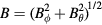 is the background equilibrium magnetic field with
  . The safety factor
  is a function of the plasma minor radius.
For the kink mode, the poloidal variation of mode amplitude is unimportant, thus neglected here. The fluctuating generalized vorticity, 
 [27], is the quantity advected by the equilibrium sheared E × B flows, not the fluctuating electrostatic potential,
  . Then, the eigenfunction of the mode in this coordinate system can be written in the form

where  is the initial radial amplitude profile of
  , i.e. the initial radial distribution of polarization charge. It is only a function of the plasma minor radius. The radial amplitude profile of
  at time t is
which appears to have been modified by the differential advection,  , induced by the sheared E × B flows. Note that
  is r-dependent. Here,
 ![$\nabla _{\bot}^{2}\hat{\varphi}=\left[{{r}^{-1}}{{\partial}_{\text{r}}}\left(r{{\partial}_{\text{r}}}\right)-k_{y}^{2}\right]\hat{\varphi}$](https://content.cld.iop.org/journals/0029-5515/57/8/086047/revision2/nfaa7975ieqn225.gif) .
.
For kink modes, the unstable region is inside of the rational surface ( ) where
  [28]. The initial radial amplitude profile of
  is assumed to be a half-Gaussian distribution function centering at the rational surface with a radial decay length of
  (the radial mode width),
  with
with  the step function. Its first and second radial derivatives can be calculated analytically by
  and
and  . The radial decay length
  is of ~1 centimeter, which is consistent with the fluctuation measurements of electron density and temperature in the pedestal region of DIII-D, indicating that EHOs are localized in the pedestal steep-pressure-gradient region with a radial width of a few centimeters, as shown by figure 10 in [16].
Substituting  and
and  expressions into the mode eigenfunction, we have

where  is the wavenumber in the y direction,
  is the poloidal wavenumber and
  is the toroidal wavenumber.
The definition of the mode frequency in the laboratory-rest frame,  , is the same as that in section 3. In a plasma with equilibrium sheared E × B flow,
  is r-dependent, since
  is r-dependent. However, the mode frequency in the plasma-moving frame,
  , is invariant with the plasma minor radius for a given eigenmode. The E × B shearing rate is given by
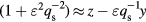
  in the cylindrical geometry and
  in the toroidal geometry [29]. The shear frequency is defined by
  [30]. Taylor expanding
  around the rational surface, we have
  . The radial gradient of
  is
is  .
.
Under the drift approximation [28], the leading order convective time derivative is given by  with
with  ,
,  the radial E × B convection velocity and
  the E × B advection velocity in the y direction. Here, positive
  is in the electron diamagnetic direction. Note that the advection by parallel flow,
  , has been neglected here. This time derivative is calculated in the reference frame moving with the fluid, thus the observed frequency is the mode frequency in the plasma-moving frame of reference. In contrast, the time derivative
  is calculated in the laboratory-rest frame of reference, thus the frequency is modified by the E × B Doppler shift. Then, we have
  and
and  . Note that in this analysis we only consider the linear problems, thus all nonlinear terms have been neglected.
The flow in a tokamak plasma is usually subsonic, i.e.  with
with  the ion thermal velocity, thus the ion inertia term,
  , is small in the equilibrium equation. Then, we have the radial force balance equation,
  [1], where
  is the equilibrium radial electric field with
  the stationary electrostatic potential, which is a flux function,
  and
and  is the toroidal and poloidal ion rotation velocity, respectively. The ion pressure gradient,
  , is usually determined by the ion thermal and particle radial transport. The radial electric field can be modified through changing the ion rotations, especially the toroidal rotation, since the toroidal rotation in a tokamak can be easily controlled by external torque sources such as NBIs.
In a tokamak, a net equilibrium flow can be written as  [31], where
 is the ion toroidal rotation frequency, which is a flux function,
  is the toroidal unit vector. Note that the incompressibility condition is satisfied,
 ![$\nabla \centerdot {{\mathbf{v}}_{0}}=K(\psi )\nabla \centerdot \mathbf{B}+\nabla \centerdot \left[{{R}^{2}} \Omega (\psi )\nabla \phi \right]=0$](https://content.cld.iop.org/journals/0029-5515/57/8/086047/revision2/nfaa7975ieqn273.gif) and the E × B flow is compressible. The parallel flow helps to keep the incompressibility. The total parallel flow is
and the E × B flow is compressible. The parallel flow helps to keep the incompressibility. The total parallel flow is  and the perpendicular flow is
  . The total toroidal rotation velocity is
 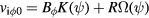 and the poloidal rotation velocity is
  . One can see that only the poloidal rotation has no coupling with the radial electric field in a helical magnetic field.
In the helical coordinate system [3], the gradient along the magnetic field line is given by  with
with  where
where  is the perpendicular magnetic perturbation. Its radial and y-direction component is
  and
and  , respectively. With the Ampère's law, we have the parallel current perturbation,
  . Note that
  , we have the parallel wavenumber along the background equilibrium magnetic field
  , where
  and
and  is the connection length. Taylor expanding
  around the rational surface, we obtain
  , its radial gradient
  and radial curvature
  .
.
In the helical coordinate system [3], the curvature drift operator becomes  with
with  and
and  the normal and geodesic curvature, respectively. Here, the average curvature is a constant of order
  .
.
4.2. Model of kink/peeling modes
The model of kink/peeling modes includes four coupled equations:


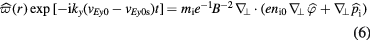
Equation (8) is the quasi-neutrality condition. Equation (9) is the parallel generalized Ohm's law, where the electron-ion collisions, electron inertia and kinetic effects such as Landau damping and trapped particles have been neglected. Equations (10) and (11) is the simplified electron and ion pressure equation, respectively.
After the well-known gyro-viscous cancellation [28], the divergence of the polarization current and gyro-viscosity current is given by

which describes the inertia of electrostatic motion. Here, the last term,  , is the K–H drive term, responsible for driving the K–H instability [17]. The equilibrium generalized vorticity
  [17] has been defined in section 2. One can see that the K–H drive in a tokamak is mainly proportional to the radial curvature of the perpendicular flow. However, the K–H instability is usually thought stable in the tokamak plasma edge due to a strong stabilization effect by magnetic shear [18]. The K–H drive will be neglected in the following eigenvalue analysis, since the purpose of this paper is not to study the effects of K–H drive.
We express the fluctuating generalized vorticity,  , in the quantities normalized by the values on the rational surface,
  ,
,  ,
,  ,
,  ,
,  is the ion density gradient length. The divergence of the diamagnetic drift gives the interchange drive,
 [28], where
  ,
,  . The system couples to the shear Alfvén wave through the divergence of the parallel current density,
  , with the first term representing the kink drive and the second term describing the field line bending [28].
After linearization and normalization, the four-coupled equations become


where  is the Alfvén frequency,
  is the Alfvén velocity on the rational surface,
  ,
,  is the magnetic surface average operator,
  ,
,  is the electron diamagnetic frequency,
  is the electron pressure gradient length,
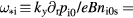
 is the ion diamagnetic frequency and
  is the ion pressure gradient length. The electron curvature drift frequency is defined by
  .
.
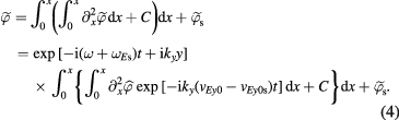
The first term in equation (13) is the inertia term; the second term is the field line bending term due to coupling to the shear Alfvén wave; the third term is the kink drive term; the fourth term is the K–H drive term and the last term is the interchange drive term. For a kink mode, it experiences only the average curvature which is usually favorable in a tokamak, therefore the interchange drive term is a weak stabilization term with  .
.
Substituting equation (15) into (14), we have

Then, substituting equations (15)–(17) into equation (13), noting that  is invariant with the plasma minor radius, we arrive at the eigenvalue equation

Note that the radial gradient and curvature of  have been neglected. This is a quadratic equation in
  . The coefficients are
The diamagnetic stabilization effect [27] has been included, since we are using the fluctuating generalized vorticity. According to the energy principle [28], we multiply the coefficients by  and calculate the radial integral,
  , over a radial range,
  , covering the whole pedestal region, e.g.
  and
and  with
with  the plasma minor radius at the last closed flux surface. Then, we obtain a quadratic equation in

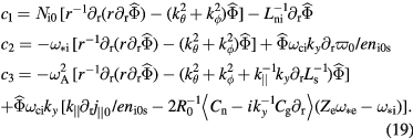
Solving this equation, we finally obtain the dispersion relation,  . Its imaginary part is the required linear growth rate.
5. Numerical linear eigenvalue analysis using DIII-D experimental data
In this section, we conduct a linear eigenvalue analysis using DIII-D experimental data in a typical QH-mode discharge with toroidal rotation velocity ramping down to zero [13].
5.1. Descriptions of the experiment and the discharge
Very recently, a new kind of QH-mode regime with increased pedestal pressure and width at low rotation has been discovered serendipitously in the DIII-D tokamak [13]. The low rotation was achieved by slowly ramping down the external injected torque during the plasma discharge through balancing the co-Ip and counter-Ip oriented external torque injection from neutral beams. A low-n broadband incoherent electromagnetic turbulence, so-called 'broadband MHD' [13], appears in the pedestal region, replacing EHOs. The low rotation leads to a reduced E × B flow shear in the pedestal with an accompanying stabilization of the EHOs and an increase in height and width of the pedestal, which is within the limits allowed by peeling-ballooning mode theory. It could be a very important discovery, since the plasmas in future fusion devices are anticipated to operate at low rotation due to large plasma inertia and limited external torque injection. Stationary operation with improved pedestal conditions but without detrimental ELMs is highly desirable for fusion energy production.
Figure 6 shows the time histories of the toroidal rotation velocity at the pedestal top and the toroidal-mode-number spectrogram in a typical discharge #163518 of this experiment. The details of this discharge have been described in [13]. The toroidal rotation velocity and radial electric field profiles were measured by a charge-exchange-recombination spectroscopy (CER) diagnostics on DIII-D [32]. The toroidal-mode-number spectrogram is the crosspower between two poloidal magnetic field fluctuation signals measured by two toroidally distributed Mirnov magnetic probes on the outer midplane wall of the DIII-D vacuum vessel. The 30° difference in the toroidal angle allows the determination of the toroidal mode number n up to 5, which is indicated by the color plotted. The color scale on the right hand side of the plot shows the relation between color and mode number. The time point for this analysis is 2.35 s as indicated by the vertical line in the plots. Some parameters at this time point, which have been used in the following analysis, are toroidal magnetic field  on the magnetic axis, major radius
  , minor radius
  , plasma internal inductance
  and poloidal beta
  .
.
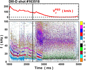
Figure 6. Time histories of the toroidal rotation velocity at the pedestal top measured by a charge-exchange-recombination spectroscopy (CER) diagnostics and the toroidal-mode-number spectrogram in a typical QH-mode discharge #163518 in DIII-D. The toroidal-mode-number spectrogram is the crosspower between two poloidal magnetic field fluctuation signals measured by two toroidally distributed Mirnov magnetic probes on the outer midplane wall of the DIII-D vacuum vessel. The 30° difference in the toroidal angle allows the determination of the toroidal mode number n up to 5, which is indicated by the color plotted. The color scale on the right hand side of the plot shows the relation between color and mode number. The vertical line at 2.35 s in the plots marks the time point for the following analysis.
Download figure:
Standard image High-resolution imageAs shown in figure 6, the toroidal rotation velocity at the pedestal top ramps down from ~100 km s− in the counter-Ip direction to zero by reducing the counter-Ip NBI power. The low-frequency coherent modes are observed in the toroidal-mode-number spectrogram at high rotation are the EHOs dominated by modes with toroidal mode number n = 1–4. Integrating the Mirnov signal over time, we have the amplitude of the poloidal magnetic field fluctuation. The n = 2 mode has the highest fluctuation level in the integrated signal at 2.35 s, suggesting that n = 2 is the most unstable mode. The dominant toroidal mode number of EHOs is typically n ⩽ 3 [6–8]. In the recent linear eigenmode analysis with M3D-C1 code, n = 2 is the most unstable mode at the experimental rotation level [16], consistent with the dominant EHO mode observed in the experiment. The EHO frequencies decrease with time as the toroidal rotation velocity decreases, mainly due to Doppler shift. The EHOs disappear at ~2.9 s, when the toroidal rotation velocity is reduced to below 50 km s−1, then replaced by a low-n broadband electromagnetic turbulence, as shown in the toroidal-mode-number spectrogram. The propagation direction of EHOs is in the counter-Ip direction, following the plasma rotation with dominantly counter-Ip NBI, whereas some low-frequency components of the broadband electromagnetic turbulence follow the plasma current direction instead, probably due to Doppler shift with reduced E × B flows at low NBI torque.
5.2. Profile data and equilibrium inputs for the analysis
The analysis focuses on the strong coherent EHOs at 2.35 s in discharge #163518. The radial kinetic profiles as shown in figures 7(e) and (f), including electron density  , temperature
  and ion density
  , temperature
  , are obtained by averaging the data points over a 100 ms time window centered at 2.35 s using a Python based profile-fitting program [33]. The equilibria used for profile fitting are produced with the EFIT [34] code based on the magnetic measurements. At each measurement time point, the data points are mapped from physical to poloidal magnetic flux coordinate and then all individually mapped data within the overall averaging time window are collected and fitted to a modified tanh (mtanh) function [35] in the pedestal region and a spline model in the core region except the ion temperature
  profile which is fitted to a spline model in the whole region. The electron density
  and temperature
  are obtained from Thomson scattering (TS) diagnostics. Impurity (carbon) density
  , ion temperature
  and radial electric field
  are obtained from CER diagnostics. The radial electric field profiles including
  (red),
  (black) and
  (blue) are shown in figure 7(c) and their corresponding shearing rates
  (red),
  (black) and
  (blue) are shown in figure 7(d). The ion density
  profile shown in figure 7(e) is calculated by
  , assuming carbon is the only impurity. The electron (ion) pressure
  (
( ) shown in figure 7(g) is taken as the product of the electron (ion) density and temperature, respectively.

Figure 7. Radial profiles of several key plasma parameters in the edge pedestal at 2.35 s in a typical QH-mode discharge #163518 on DIII-D. (a) safety factor q, (b) flux surface averaged current density  , (c) radial electric fields, including
  (red),
  (black) and
  (blue), (d) corresponding shearing rates,
  (red),
  (black) and
  (blue), (e) electron density
  (black) and ion density
  (red), (f) electron temperature
  (black) and ion temperature
  (red), (g) electron pressure
  (black) and ion pressure
  (red), (h)
  (blue),
  (black),
  (red) and
  (blackish green), where the toroidal mode number n has been set to 1.
Download figure:
Standard image High-resolution imageThe experimentally measured total pressure profile is used as a constraint for a kinetic equilibrium reconstruction, which is the sum of the measured electron and ion pressures and the fast ion pressure calculated using the Monte Carlo NUBEAM [36, 37] module in the ONETWO [38] transport code. The flux surface averaged toroidal current density in the core plasma is determined from motional Stark effect (MSE) [39] measurements, while in the pedestal region, it is derived from the sum of the parallel bootstrap current given by the Sauter expression [40, 41], the neutral beam driven current computed using NUBEAM and the Ohmic current density. The Ohmic current density is determined from the neoclassical expression for the resistivity with a loop voltage, which is assumed spatially constant and adjusted to give a net plasma current matching the measured total plasma current. Iterations are taken in the reconstruction process wherein the pressure profile is remapped to poloidal flux coordinate and the pedestal current density is also recalculated.
The final safety-factor q profile and flux surface averaged current-density  profile from the kinetic equilibrium are shown in figures 7(a) and (b), respectively. According to the q profile, the q = 7 rational surface is located in the steep current-density gradient region where the kink/peeling mode is unstable, marked with purple vertical lines in figure 7, and the current-density gradient at q = 6 rational surface is positive where the mode is stable. Figure 7(h) shows
  (blue),
  (black),
  (red) and
  (blackish green) profiles, where the toroidal mode number n is set to 1.
5.3. Linear eigenvalue analysis using the new model
A linear-stability eigenvalue analysis of the dominant kink/peeling mode in the edge pedestal is performed for the discharge at t = 2.35 s using the new model developed in section 4. The new mechanism for destabilizing kink/peeling modes by E × B flow shear is the flow-shear-induced radial expansion of the mode structures radially away from the rational surface.
Firstly, we substitute the DIII-D data into the model and solve the eigenvalue equation, equation (20), numerically without radial expansion (no effect of sheared flows), i.e. t = 0 in equation (6). The initial radial amplitude profile of the mode electrostatic potential structures,  , is a half-Gaussian distribution function centering at the rational surface with the radial decay length,
  , the only undetermined parameter. We search in the parameter space of
  to maximize the linear growth rate,
  , for each toroidal mode number, n. For a given n, the mode is unstable only when a positive linear growth rate can be found, otherwise the mode is linearly stable and the corresponding parameter
  cannot be determined. This approach is reasonable, since in reality the mode that finally appears in the experiments is the most unstable mode for each n.
The K–H drive term,  , in expression (19) has been neglected, since it is not the focus of this paper. One can see that there is no
  dependence in expression (19) except through the K–H drive term. Therefore, in the model, without the effect of radial expansion, there is nowhere the sheared E × B flows can influence the solution of the eigenvalue equation. The sheared E × B flows just introduce a Doppler shift, which modifies the mode real frequency,
  , in the laboratory-rest frame of reference.
The stability-analysis result without radial expansion is shown in figure 8 with the magenta curves. The linear growth rate,  , in figure 8(a) indicates that the modes are unstable in the low to intermediate n range, n = 2–9, consistent with the previous stability-analysis results of kink/peeling mode with the ideal-MHD code ELITE [4, 9, 16]. The most unstable mode is n = 6, which is considerably higher than the toroidal mode number of the dominant mode observed in the experiment, i.e. n = 2. The peak linear growth rate is
  . The real frequency in the plasma-moving frame of reference,
  , in figure 8(b), shows a nearly linear dispersion relation in the ion diamagnetic direction (negative). The radial decay length,
  , of the mode electrostatic potential structures in figure 8(c) is in the range of 3–5 mm, peaking with
  at n = 3. The radial amplitude profile of the mode electrostatic potential structures for n = 3 mode is shown in figure 9 with the dark yellow curve, which is a half-Gaussian distribution function,
  . The radial width of the mode is generally comparable with the pedestal width.

Figure 8. Results of a linear eigenvalue analysis of kink/peeling mode using the new model with DIII-D data at 2.35 s in a typical QH-mode discharge #163518, including (a) linear growth rate  , (b) real frequency in the plasma-moving frame of reference
  , (c) radial decay length
  of the initial mode electrostatic potential structures. The magenta curves show the results without radial expansion effect, i.e. at t = 0, no effect of sheared flows. Other curves show the results with radial expansion effect, i.e. at
  , with different radial electric field profiles as shown in figure 7(c),
  (red),
  (black) and
  (blue).
Download figure:
Standard image High-resolution image
Figure 9. Radial amplitude profile of the mode electrostatic potential structures for n = 3 mode without radial expansion effect, i.e. at t = 0, no effect of sheared flows (dark yellow), which is a half-Gaussian distribution function,  . The real (blue) and imaginary (red) parts of the radial amplitude profile of the mode electrostatic potential structures for n = 3 mode with radial expansion effect, i.e. at
  . The radial electric field profile,
  , measured in the DIII-D experiment has been used in this analysis.
Download figure:
Standard image High-resolution imageWhen the radial expansion is taken into account, the radial amplitude profile of the mode electrostatic potential structures,  , evolves with time according to equation (6), and is no longer a simple half-Gaussian distribution function. It can be solved analytically or numerically through radial integrations of the Poisson's equation with the radial decay length,
  , fixed at the value at t = 0, as described in section 3 by expression (4). Note that here the integrations are conducted in a helical coordinate system, we then have
The real and imaginary parts of  for n = 3 mode at
  are shown in figure 9, where
  is the shear Alfvén time calculated on the rational surface. Compared with the profile at t = 0, i.e. the half-Gaussian distribution function shown with the dark yellow curve, the real part of the profile at
  , shown with the blue curve, appears to be broadened and enhanced in amplitude with a long tail expanding radially significantly away from the rational surface. The imaginary part reflects a tilt of the mode electrostatic potential structures with a radial phase shift,
 ![$\arctan \left[{{\hat{\varphi}}_{Im}}(r)/{{\hat{\varphi}}_{\operatorname{Re}}}(r)\right]$](https://content.cld.iop.org/journals/0029-5515/57/8/086047/revision2/nfaa7975ieqn409.gif) , radially increasing away from the rational surface, as shown in figure 5. This profile change is induced by E × B flow shear, as indicated in expression (21), and it will have significant influence on the linear growth rate of the kink/peeling mode, as shown in figure 8(a).
, radially increasing away from the rational surface, as shown in figure 5. This profile change is induced by E × B flow shear, as indicated in expression (21), and it will have significant influence on the linear growth rate of the kink/peeling mode, as shown in figure 8(a).
This theory successfully explains the observations that EHOs always appear with only a few coherent low-n harmonics and that the wavenumber spectrum is significantly broadened at low E × B flow shear. We scan the equilibrium radial electric field,  , by multiplying a factor from half to two times of the measured value, which changes the E × B flow and flow shear simultaneously, as shown in figures 7(c) and (d), but with other parameters fixed. The kink/peeling modes appear to be destabilized at low n, but stabilized at high n and intermediate n by the E × B flow shear. With increasing sheared flows the toroidal mode number of the most unstable mode moves towards low n, i.e.
  with
with  ,
,  with
with  and
and  with
with  . The unstable modes with
  are
are  = 2–4, which are generally consistent with the experimental observations in figure 6. The n = 1 mode is stable in this analysis, since it is already stable at t = 0 (no effect of sheared flows). Note that the n = 1 mode is stable only for this particular case and it is unnecessarily stable for other profiles. The peak linear growth rate decreases with increasing sheared flows, which may facilitate the saturation, since a saturation is usually achieved when the nonlinear damping rate balances the linear growth rate. A smaller linear growth rate is easier to be balanced. In addition, the real frequencies (negative) are slightly reduced with increasing sheared E × B flows, as shown in figure 8(b).
In summary, these stability-analysis results indicate that with strong sheared flows, only a few low-n modes remain unstable, and with reduced sheared flows, the toroidal mode number spectrum is broadened, consistent with the observations of coherent EHOs at high rotation and a transition to broadband electromagnetic turbulence at low rotation in the recent DIII-D experiments [13].
To further study the effect of E × B flow shear on the mode stability, the equilibrium radial electric field,  , is shifted radially outwards from negative shear to positive shear on the rational surface step by step, as shown in figure 10, but with other parameters fixed. The results of linear stability analysis are shown in figure 11 with different colors corresponding to different shifts. When
  is shifted radially, the E × B shearing rate,
  , on the rational surface is reduced, until the blue curve where the rational surface nearly passes through the flat bottom of the
  well. Indeed, the broadest toroidal mode number spectrum is obtained with the smallest
  , as shown with the blue curve in figure 11(a), and as expected, the toroidal mode number spectrum is gradually broadened as
  decreases. With positive shear, as shown with the magenta curve in figures 10 and 11, the toroidal mode number spectrum becomes narrow again, demonstrating that the effect is independent of the sign of the flow shear, consistent with the experimental observations of EHOs at both negative and positive rotations [8].

Figure 10. Equilibrium radial electric field profile,  , measured by CER diagnostics at 2.35 s in a typical QH-mode discharge #163518 of DIII-D experiment (black), and the shifted
  profiles, radially outwards with each step by 0.01. ρ is the normalized minor radius. The dashed vertical line shows the radial location of q = 7 rational surface.
Download figure:
Standard image High-resolution image
Figure 11. Results of a linear eigenvalue analysis of kink/peeling mode using the new model with DIII-D data at 2.35 s in a typical QH-mode discharge #163518, including (a) linear growth rate  , (b) real frequency in the plasma-moving frame of reference
  , (c) radial decay length
  of the initial mode electrostatic potential structures. Different colors correspond to different equilibrium radial electric field profiles,
  , as shown in figure 10.
Download figure:
Standard image High-resolution image
6. Discussions and summary
6.1. Summary of new findings
This paper is motivated by recent observations in the DIII-D tokamak that coherent EHOs in QH-mode plasmas at high rotation (and hence high E × B flow shear at the plasma edge) changes into a broadband electromagnetic turbulence in the pedestal region at low rotation. We analyze and identify a new destabilization mechanism for low-n kink/peeling modes in the presence of strong E × B flow shear, separate from the K–H drive [17]. Our analysis indicates that the differential advection of mode vorticity by sheared E × B flows modifies the radial distributions of the mode generalized vorticity,  [27], the mode polarization charge. This in turn causes a radial expansion of the mode electrostatic potential structures, an increase of field line bending away from the mode rational surface, and a reduction of inertial stabilization. These in turn enhance the kink drive as the parallel wavenumber increases significantly away from the rational surface where the magnetic shear is also strong. The pedestal fluctuation measurements of electron density and temperature in DIII-D [16] indicate that the EHOs exhibit rather broad radial structure, covering the whole pedestal region or even extending inward beyond the pedestal. The predicted radial expansion of the mode structure is consistent with this observation.
Field line bending can result from the kink drive, i.e.  , which in turn is proportional to
  , i.e.
  , as shown in [28]. In ideal-MHD, the field lines are frozen in the fluid, the radial expansion of the mode electrostatic potential,
  , will lead to field line bending radially,
  , driven by radial E × B convection away from the rational surface. In the presence of magnetic shear, the angle between the mode structure and the background field line increases as the mode structure extends radially away from the rational surface. That is, the effective parallel wavenumber,
  , increases with x. Because of the field line bending, the equilibrium current-density gradient has a projection along the magnetic field lines,
  . This increases the kink drive at radial locations significantly away from the rational surface. In addition, the radial expansion reduces the radial curvature of the electrostatic potential structures,
  , reduces inertial stabilization, and thereby increases the effective linear growth rate of the kink mode.
The physics effect of the radial expansion is illustrated with 2D fluid model in section 2 and analyzed in section 3. The equilibrium E × B flow shear causes a radial expansion of the mode structure through the poloidal advection of the mode generalized vorticity, which is the polarization charge,  . This in turn introduces an increasing radial phase shift, modifies the radial distributions of mode polarization charge, modifies the radial curvature profiles of the mode electrostatic potential, and leads to radial mode expansion, as illustrated in figures 3–5.
On a longer timescale during mode growth,  , the radial expansion would appear periodically with a frequency of
  , when the mode structure shifts beyond a half-wavelength poloidally. However, this is prevented in our case, since the linear growth rates are usually much larger than the shear frequency,
  . Thus, the radial expansion continues through the period of mode growth, until nonlinear effects of the kink/peeling modes set in.
To identify the mechanism of kink/peeling mode destabilization and the resulting variations in mode behavior from different E × B flow shear, kink/peeling mode is analyzed in a helical coordinate system [3] in section 4. A linear eigenvalue analysis is carried out in section 5 for a DIII-D QH-mode discharge (#163518) [13]. The eigenvalue analysis has successfully reproduced the experimental observations that, at high E × B flow shear, only a few low-n modes remain unstable, while at low E × B flow shear, unstable modes in a broad wavenumber spectrum is obtained. These results are consistent with the observation in recent DIII-D experiments [13] of coherent EHOs at high rotation (and hence high E × B flow shear at the plasma edge) and a transition to broadband electromagnetic turbulence at low rotation. MHD simulations indicate that modes with a broad wavenumber spectrum in the linear simulations usually will evolve into broadband turbulence in the nonlinear simulations due to significantly enhanced mode-mode couplings compared to a narrow wavenumber spectrum [17, 19, 27]. Our results are further consistent with the kink/peeling mode properties revealed in simulations using the ideal-MHD codes ELITE [4] and MINERVA [14], and more recently using MHD codes M3D-C1 [16] and BOUT++ [17, 19]. Finally, as demonstrated in figure 11, this destabilization effect is shown to be independent of the sign of flow shear, consistent with the experimental observations of EHOs at both negative and positive rotations [8].
The improved understanding of the driving mechanisms of EHOs and broadband electromagnetic turbulence could facilitate the access to the QH-mode regime in future fusion plasmas to prevent the kink/peeling mode induced collapses—the large ELMs, in subsequent nonlinear development.
6.2. Future work
Only linear stability has been analyzed in this paper. The radial mode structure, as shown in figure 9 with the blue curve, as well as the radial mode width in our linear analysis, are consistent with those of EHOs observed by fluctuation diagnostics in experiments, as shown by figure 10 in [16]. However, verification of the veracity of this EHO mechanism will require analysis of the nonlinear evolution of low-n kink/peeling modes in the pedestal region. These will be addressed in future publications.
For example, the radial expansion of mode structures identified here may increase the radial extent of mode-driven transport as the mode advances into the nonlinear phase. This may provide an explanation for the observation that localized EHOs in the pedestal region may prevent impurity accumulation in the plasma core region by exhausting impurities in the pedestal region. Recently, a careful impurity-transport analysis on DIII-D [42] indicated that the impurity confinement time in QH-mode is comparable to that in ELMy H-mode, suggesting that EHOs may exhaust impurities as effectively as large ELMs.
Furthermore, E × B flow shear break the mode symmetry across the rational surface [43]. This effect has been studied extensively regarding small-scale turbulence [44–47]. It was suggested that the E × B flow shear could shift the peak amplitude of the mode eigenfunction, ![$\hat{\varphi}(x)={{\hat{\varphi}}_{\text{A}}}\exp \left[-{{(x-\xi )}^{2}}/2{{\lambda}^{2}}\right]$](https://content.cld.iop.org/journals/0029-5515/57/8/086047/revision2/nfaa7975ieqn444.gif) , radially away from the rational surface by a distance
, radially away from the rational surface by a distance  in a plasma with significant equilibrium density and temperature gradients [43]. The radial distance of shift generally increases with the shear frequency,
  . This can break
  versus
  mode symmetry (i.e. a dynamical preference for one sign of
  ) in the presence of E × B flow shear, thus introducing a net momentum source needed to cause the so-called 'intrinsic rotation' [43], independently of externally applied torque. Can this effect be applied to the large-scale MHD modes? Our results suggest that the kink/peeling mode could be further destabilized by the symmetry breaking. The strength of this mechanism relative to that of mode radial expansion will be addressed in future publications.
Acknowledgments
This work was supported by National Magnetic Confinement Fusion Science Program of China under Contracts No. 2015GB101000 and No. 2013GB106003 and National Natural Science Foundation of China under Contracts No. 11575235, No. 11422546, and No. 11321092 and Key Research Program of Frontier Sciences, CAS, Grant No. QYZDB-SSW-SLH001 and U.S. Department of Energy under Contract DE-FC02-04ER56498.