
Abstract
Hadrontherapy is an innovative radiation therapy modality for which one of the main key advantages is the target conformality allowed by the physical properties of ion species. However, in order to maximise the exploitation of its potentialities, online monitoring is required in order to assert the treatment quality, namely monitoring devices relying on the detection of secondary radiations. Herein is presented a method based on Monte Carlo simulations to optimise a multi-slit collimated camera employing time-of-flight selection of prompt-gamma rays to be used in a clinical scenario. In addition, an analytical tool is developed based on the Monte Carlo data to predict the expected precision for a given geometrical configuration. Such a method follows the clinical workflow requirements to simultaneously have a solution that is relatively accurate and fast. Two different camera designs are proposed, considering different endpoints based on the trade-off between camera detection efficiency and spatial resolution to be used in a proton therapy treatment with active dose delivery and assuming a homogeneous target.
Export citation and abstract BibTeX RIS
1. Introduction
Hadrontherapy is a radiation therapy modality in which ions, namely protons and carbon ions, are used to treat tumours. The energy deposition along the path of these charged particles is characterised by a pronounced increase followed by a steep decrease close to the end of the path—the Bragg peak—which allows for a higher physical dose conformality in the tumour while sparing the healthy tissue. An additional advantage of hadrontherapy is the enhanced relative biological effectiveness (RBE) in respect to the therapy with photons. The said advantage is small for protons but noteworthy for carbon ions (Paganetti et al 2002, Schardt et al 2010).
Nevertheless, uncertainties in the ion range may pose some issues in achieving the desired treatment quality. For instance, the particles used are greatly affected by tissue density changes when compared to photons, thus extra care must be taken in both the planning and delivery of the treatment. The current practise is to use safety margins (Albertini et al 2011, McGowan et al 2013) in order to account for the multiple possible sources of uncertainties associated to a typical hadrontherapy treatment (Paganetti 2012). As a consequence, the theoretical advantage of dose conformality and the possibility of having reduced margins around the target volume due to the limited particle range are not fully exploited. As recently shown in a public survey conducted during the 54th annual meeting of the American Association of Physicists in Medicine, 33% of the attendees selected the range uncertainties associated with proton therapy as the main obstacle to this treatment modality becoming mainstream (Freeman 2012).
In order to try to overcome such drawbacks, ion range monitoring techniques are of paramount need (Knopf and Lomax 2013). Currently, only positron emission tomography (PET) is implemented in clinical routine but other techniques may prove useful, namely the ones relying on prompt-gamma detection. Both exploit the ion range information provided by secondary particles created after inelastic collisions between the incident ions and the nuclei in the body of the patient (Schardt et al 2010).
Prompt-gamma monitoring development has been so far focused in two categories of possible solutions and both consider the detection of prompt gammas orthogonally to the beam axis in order to maximise the correlation between the detected photon and the position along the ion path. The first solution is to use a device with electronic collimation, e.g. a Compton camera (Phillips 1995, Peterson et al 2010, Richard et al 2011, Robertson et al 2011, Mackin et al 2012), while the second is based on passive collimation. For the latter, two main possibilities have been studied, either a knife-edge slit camera (Bom et al 2012, Smeets et al 2012) or a parallel multi-slit one (Min et al 2006, Testa et al 2008, Testa et al 2010, Roellinghoff et al 2014). This work deals with the optimisation of a device of the latter type. Despite the fact that other studies have already addressed the optimisation of parallel multi-slit collimators for this application (Cambraia Lopes et al 2012, Min et al 2012), the present study is assumed to be distinct due to the emphasis given to the use of time-of-flight (TOF) applied to this technique. Moreover, experimental TOF information is used to support and benchmark the set of methods used throughout this study. The importance of TOF has been shown for both proton (Biegun et al 2012, Roellinghoff et al 2014) and carbon ion (Testa et al 2008, Testa et al 2010) modalities, for which its use enhances the performance of such cameras by ameliorating the signal-to-background ratio (SBR). In a first approximation, using TOF improves the precision in finding ion range shifts by a factor proportional to the square root of the background reduction (Roellinghoff et al 2014).
The use of passive collimating devices for medical imaging is an established procedure when there is the need to collimate either emitted or transmitted radiation, mainly for diagnostic purposes. As an example, for nuclear medicine imaging, the optimisation of passive collimators relies on geometrical and photon attenuation considerations since the energy of the incoming particle is known. In any case, it is not possible to have energies higher than the one characteristic of the radioisotope injected in the patient. Moreover, there is no concern about the background since the only source of radiation is the patient. A comprehensive overview on this topic was made by Gunter (2004).
The use of passive collimating systems in hadrontherapy, however, needs to respect different conditions in order to be able to take advantage of the information provided by prompt gammas. The energy of the emitted prompt gammas is not fixed, possessing an energy spectrum ranging up to more than 10 MeV (Polf et al 2009). On the other hand, the treatment room contributes with radiation background due to e.g. inelastic interactions of charged particles and interactions of neutrons in the delivery machine nozzle and room walls. In that sense, even the collimator itself may act as a secondary source of radiation.
A key aspect of hadrontherapy monitoring is to be able to find the ion range inside the patient. This means that the aim of the prompt-gamma camera is to detect edges corresponding to the entrance rise and the fall-off in the prompt-gamma longitudinal profile. For this purpose, unlike for nuclear medicine imaging, a good spatial resolution is not a priori required. Likewise, it is not mandatory to have three-dimensional information since mainly the longitudinal ion path is relevant. One may consider the potential usefulness of retrieving three-dimensional images, however such a task is outside the scope of this paper. Therefore, there is no need to ponder about a multi-hole collimator system as often used in nuclear medicine, but rather focus on a multi-slit one with parallel slabs and positioned orthogonally to the beam axis.
The present work is based on Monte Carlo simulations, thus there was the need to verify their accuracy in this context, which was achieved by a benchmarking with experimental data. In the optimisation process, the TOF technique is used in order to achieve a better camera performance due to the improved SBR. Moreover, this study aims not only at finding a solution that yields a good performance, but also at understanding the trends of the camera geometry that drive its performance. The following sections present the methods employed to optimise a parallel multi-slit camera, with emphasis on the collimator, the expected performance based on Monte Carlo simulations, and on a discussion about the potentiality and possible limitations of using such a collimated camera for hadrontherapy monitoring purposes. Although this work is mainly focused on proton therapy monitoring and on data coming from experiments with protons, all the procedures followed should also be applicable to other ion species, namely carbon ions.
2. Methods
The optimisation of a parallel multi-slit camera is not a trivial procedure mainly due to the complexity of the physical processes taking place during a hadrontherapy treatment, as shown in the previous section. The most adequate strategy to optimise a device in this scenario is based on Monte Carlo tools. However, only if the trends in the optimisation process are understood, i.e. how the variation in each parameter influences the final design and its performance, it is possible to drive further developments.
Assuming that the physical models implemented in Monte Carlo tools are accurate enough, one could attain a high level of accuracy in the expected performance. Nevertheless, Monte Carlo simulations require large amounts of computing time, which leads to a lack of flexibility of the optimisation process for e.g. the fine tuning of the camera geometrical parameters. Such a flexibility is crucial if e.g. some mechanical constraints are met during the construction phase and a fast adjustment of the camera design is needed.
In this context, the present work comprises three stages. The first addresses a benchmarking of the Monte Carlo tool chosen in order to select the best physical models for this application. The second stage is focused on the optimisation by means of Monte Carlo simulations. Since there is no a priori knowledge about the parameters that influence the camera performance the most, it was decided to simulate multiple random geometries constrained by meaningful boundaries. After this point, it is possible not only to choose the camera geometry with the best performance among the ones simulated, but also to understand the trends in the geometrical parameters that impact its performance the most. Finally, the third stage uses all these simulations as a training data set for a multivariate regression analysis in order to have an analytical tool able to predict camera performances. Such a tool is not intended for further optimisation of the device but rather to provide fast and accurate results within the region considered in the training. One could argue that this parametrisation could be used to achieve better camera performances, however it would be at the cost of extrapolation and it would always require simulations to cross-check the result.
The Monte Carlo simulations were carried out with the Geant4 toolkit (Agostinelli et al 2003), version 9.6.p01, and the regression analysis was made using a built-in library in ROOT framework (Brun and Rademakers 1997) called TMultiDimFit.
Unless otherwise stated, all results presented herein only consider events with an energy deposition higher than 1 MeV in order to improve the signal to background ratio of prompt gammas.
2.1. Geant4 benchmarking
The Geant4 benchmarking comprised two steps, the first one to rule out the most inaccurate hadronic physics models and the second one to make an in-depth study of the Geant4 model outcomes. The decision to do the first step was to avoid spending too much computing resources with models that could be excluded in a more simplistic analysis.
Geant4 is a toolkit in which the user is responsible for selecting the most appropriate physics models for the given problem. The electromagnetic models available should not have a critical impact on the results since their overall precision is around a few percent (Amako et al 2005, Lechner et al 2010). On the other hand, the hadronic models, especially those concerning the prompt-gamma emission yields, may influence significantly the outcome, as already demonstrated by Le Foulher et al (2010) and Dedes et al (2014) for the case of carbon ion irradiation. Although these studies deal essentially with carbon ions, the latter also suggests an overestimation of prompt-gamma yields for proton irradiation. Therefore, a comprehensive study about Geant4 limitations pertaining to protons as primary particles is essential to not only be able to select the most adapted set of physical models for the simulations, but also to discuss more thoroughly the expected camera performance.
User-defined physics lists were utilized in order to test a broad set of physics models, raising questions concerning user-related errors in the physics list definition. As a consequence, each step of Geant4 benchmarking also includes two built-in reference physics lists (i.e. defined by the Geant4 developers) to ensure the absence of physics models inconsistencies that could be explained by user-related errors.
2.1.1. First selection of physical models.
A 160 MeV proton beam impinging on a cylindrical polymethyl methacrylate (PMMA) target was simulated for several hadronic physics models (tables 1 and 2). The target has a radius of 75 mm and a length of 200 mm. The same target is used throughout the present paper for both simulations and experiments. In this simulation the information concerning all photons able to escape the target is stored in a file for further analysis. By applying an angular acceptance constraint on the data, one is only able to select the photons that have the highest probability of being detected by a hypothetical collimated camera. These prompt gammas are, in the context of this monitoring technique, the signal of interest and it is utterly fundamental to have the best description of the signal. The outcomes of the simulations with the different models are then compared and those considered the best for this application are selected for the next step.
Table 1. Naming conventions for each set of Geant4 physics models tested. For simplicity reasons the designation of each model in this table was abbreviated, thus QMD corresponds to G4QMDReaction, BC to G4BinaryCascade, BERT + OWN to G4CascadeInterface (Bertini cascade) with its own pre-equilibrium phase implementation, and BERT + PRECO to G4CascadeInterface using G4PreCompoundModel for pre-equilibrium instead of the built-in implementation in the G4CascadeInterface. By default, BC is followed by the G4PreCompoundModel while QMD has no equilibrium phase. The de-excitation phase is common to all the collision models. Apart from the ones described here, the reference physics lists QGSP_BIC_HP and QGSP_BERT_HP were also used.
| Name | Hadronic inelastic | |||
|---|---|---|---|---|
| Protons | Neutrons | Others | ||
| > 20 MeV | < 20 MeV | |||
| phys1 | BC | BC | ||
| phys2 | BERT + OWN | BC | ||
| phys3 | BERT + OWN | BERT + OWN | ||
| phys4 | BERT + PRECO | BERT + OWN | ||
| phys5 | BERT + PRECO | BERT + PRECO | ||
| phys6 | QMD | BC | G4NeutronHPInelastic | QMD |
| phys7 | QMD | BERT + OWN | ||
| phys8 | QMD | QMD | ||
| phys9 | BC | BERT + OWN | ||
| phys10 | BC | BERT + PRECO | ||
| phys11 | BERT + PRECO | BC | ||
Table 2. Other Geant4 simulation settings common to all user-defined sets of physical models tested.
| EM | Hadronic elastic | Other processes |
|---|---|---|
| G4DecayPhysics | ||
| G4EmStandardPhysics_option4 | G4HadronElasticPhysicsHP | G4EmExtraPhysics |
| G4RadioactiveDecayPhysics |
Among the hadronic physics models selected for this first selection, the Bertini cascade model with its own pre-equilibrium and de-excitation implementations is considered (BERT + OWN in table 1). This model is known for being less accurate for proton dose calculations than Binary cascade (see e.g. Jarlskog and Paganetti 2008) and to have too simplistic of an approach for modelling prompt-gamma emission (Verburg et al 2012). However, such a model was included in this first benchmarking in order to verify to what extent these issues may affect the longitudinal prompt-gamma emission profiles.
2.1.2. In-depth study of selected physics lists.
After selecting the most promising sets of physical models, Geant4 simulation outcomes were compared with experimental data. For a more thorough analysis TOF data was used, which allowed for the analysis of both background and signal behaviours by comparing an experimental TOF spectrum with a simulated one.
The experiment was conducted at the Westdeutsche Protonentherapiezentrum Essen clinical facility (WPE, Essen, Germany). A 160 MeV proton beam was implanted in the cylindrical PMMA phantom described in the beginning of this section. A cylindrical cerium-doped lanthanum(III) bromide (LaBr3:Ce) detector with a 1'' diameter and 2'' length was placed at 505 mm from the beam axis immediately behind a tungsten-alloy collimator, which had a slit of 4 mm. The TOF stop signal was given by the high frequency signal of the cyclotron running in pulsed mode with a time structure of approximately 1 ns pulse (rms) every 9.4 ns (∼ 106 MHz). The circular beam spot was around 5 mm rms at isocentre with a Gaussian spatial beam distribution (Grevillot et al 2011). A schematic illustration and a picture of this experiment can be observed in figure 1.
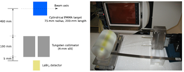
Figure 1. A schematic illustration (left, not to scale) and a picture (right) of the WPE 160 MeV protons experiment.
Download figure:
Standard image High-resolution image2.2. Simulation of random camera geometries
The purpose of simulations was to obtain the longitudinal profile resulting from a given set of geometrical parameters and to estimate the corresponding precision. This allows for (1) finding a camera design able to yield a good performance (precision), (2) trying to understand the trends that drive precision, and (3) yielding the input for the regression analysis by relating the precision obtained for a given simulated profile and the different geometrical parameters. The simulations of the random geometries were carried out with only the most accurate set of physical models among the ones tested.
The concept of precision in this context has already been extensively described elsewhere (Roellinghoff et al 2014) and it is related to the uncertainty in finding the true value of the position of the prompt-gamma profile fall-off close to the end of the ion range. It is also intrinsically associated with the overall performance of the camera in estimating the ion range for a given number of ions. The method for retrieving the precision relies on having a reference profile with high statistics which, in turn, is fit by a non-uniform rational B-spline (NURBS) function in the region of the profile fall-off. The high statistics profile is then sampled into lower statistics profiles corresponding to the expected statistics of a given number of incoming protons and the NURBS function is used to fit such a low-statistics profile. This function has only one degree of freedom that corresponds to the beam axis direction, thus yielding a deviation from the reference profile mainly driven by statistical fluctuations. The process is repeated multiple times and a histogram of these deviations is built. Afterwards, the standard deviation of this histogram is stored in a second one and the process is repeated through several iterations. The precision is then the mean value of the second histogram and the precision error (statistical) corresponds to one standard deviation.
Although the notion of precision was described in terms of the fall-off position, the same method can be applied to the prompt-gamma profile entrance rise, thus retrieving the target entrance position. With the combined information from the entrance and fall-off positions it is possible to estimate the prompt-gamma profile length. All these quantities are essential to understand how to use this technique in a clinical scenario. Ultimately, the goal is to determine the ion range inside the target, which is correlated to the prompt-gamma profile length, but a reference measurement of the point where the incoming beam enters the patient is also mandatory. Unless stated otherwise, precision refers to the precision in finding the position of the prompt-gamma profile fall-off.
The detector considered for simulations was a bismuth germanium oxide (BGO) monoblock with dimensions of 50 mm3 × 100 mm3 × 250 mm3 (x, y, z and considering the beam axis as the z-axis). The expected time resolution of these detectors is around 3 ns at full-width half maximum (FWHM). For simulations, a TOF selection window of 4 ns centred on the prompt-gamma peak was applied. The position of each event in the scintillator is estimated by the energy-weighted position of interaction. The collimator material was set to be the tungsten alloy used for some of the experiments (DENSIMET® 185). In order to avoid any edge effect in the detected events, the collimator is higher and longer than the detector. Care was taken to always have slits with the same size even at the borders. That is the reason why, in figure 2, the collimator length has a minimum of 300 mm and not a fixed value. The length of the collimator and the number of slits depend on the randomly sampled width of slits and slabs. The ranges for the random sampling of each geometrical parameter are presented in table 3.
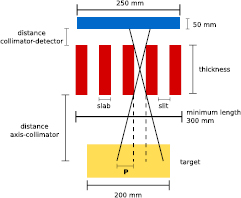
Figure 2. Schematic representation of the geometry used for the simulations (not to scale). The designations used in this figure are self-descriptive except for the geometrical parameter P that refers to the geometrical penumbra of a slit.
Download figure:
Standard image High-resolution imageTable 3. Ranges of values considered for each geometrical parameter.
| Geometrical parameter | Range (mm) |
|---|---|
| Slit width | [0.5–7.5] |
| Slab width | [0.5–7.5] |
| Collimator thickness | [50–200] |
| Distance from beam axis to collimator front face | [300–1000] |
| Distance from beam axis to detector front face | [360–1060] |
Another important remark is the potential influence of the spatial resolution on the camera performance. This point is not well known yet and requires an extensive study to understand it, which is outside the scope of the present work. However, it is acknowledged by the authors that it may play an important role in the camera performance (further discussion in section 4). In this context, it is also not clear how spatial resolution should be defined. Again, a detailed study would probably be needed for determining the most meaningful quantity and the retrieval method. Nevertheless, such a quantity should be correlated with the geometrical field of view (FOV) of the collimator on the target (slit width plus two penumbra regions estimated by the geometrical parameters of the camera). Thus, the optimisation includes a constraint on the geometrical FOV, which cannot be greater than 25 mm. This value was estimated based on the FOV of previous single-slit experiments made by our collaboration and published elsewhere (Roellinghoff et al 2014). Moreover, one of the goals of this camera is to be able to monitor ion ranges as short as a few centimetres.
Additional constraints were implemented in order to ensure that the FOV from neighbouring slits overlaps in the target. Such a constraint guarantees that the entire target around the beam range is seen through the slits of the collimator. The study of an optimal overlap was considered as being outside the scope of this work.
During the analysis of the simulated geometries a binning equal to the slit width plus the slab width (i.e. the collimator pitch) was considered for the longitudinal profiles.
In total, 14730 random geometries were simulated. A schematic representation of the geometry used for the simulations can be seen in figure 2.
2.3. Monte Carlo data analysis
The Monte Carlo data were analysed in terms of the device geometrical parameters and their relation with the precision. In order to further understand the trends driving the precision, four additional parameters were used: (1) the FOV, (2) the collimator pitch, (3) the collimator weight, and (4) the collimator fill factor. All the definitions except that of the collimator weight can be seen in equations (1)–(3). In these equations, the naming of the parameters follows the same convention as for figure 2 except for axisColl which refers to the axis-collimator distance.


The calculation of the weight of the collimator assumes a device with at least 30 cm width, but in a way that slabs always have the same size (i.e. the slabs at the extremities are not cut to obtain exactly a 30 cm-long collimator).
Finally, this analysis assumed the expected statistics for a hypothetical distal pencil beam in an active delivery system with 5 × 10⁸ protons, which somewhat overestimates what can be expected during a real treatment. The number of protons of a typical spot in a distal layer for a prostate treatment is of the order of a magnitude of 1 × 10⁸ (Grevillot et al 2012, Smeets et al 2012, Roellinghoff et al 2014). The relatively large number of protons chosen had the intention of completely avoiding the issue of outliers due to low-statistic profiles (Roellinghoff et al 2014) or other statistical artefacts. Nevertheless, as already discussed by Roellinghoff et al, the precision in an outliers-free region is proportional to the inverse of the square root of the number of protons, so any camera optimised for high statistics should remain optimal for lower statistics at least down to a number of protons for which statistical artefacts are negligible. By comparing the volume of the experimental (Roellinghoff et al 2014) and simulated detectors (this work), we estimate that the minimum number of protons for an outliers-free region for the present work is around 4 × 10⁷ protons.
2.4. Multivariate regression analysis
The regression analysis was performed using a built-in routine available in the ROOT framework called TMultiDimFit. This routine addresses the problem of multidimensional fits in physical sciences and it is an extension of the least squares fitting to higher orders by relying on polynomials (Wind 1972, ROOT team 2013). In order to use it, one needs to select appropriate initial parameters. When it is expected that the data should follow a given theoretical description, the parameters may be defined accordingly. However, for this application there was no clear idea of a mathematical model that could be used. The most problematic parameters in this case are the maximum number of polynomials in the final function and the maximum order of each polynomial. Therefore, it was decided to randomly select those parameters based on meaningful ranges inferred from the documentation and examples (ROOT team 2013). Those ranges are shown in table 4.
Table 4. Ranges of values considered for the two TMultiDimFit parameters studied.
| Parameter | Range |
|---|---|
| Maximum number of terms in each polynomial | [50–150] |
| Maximum polynomial order | [3–10] |
The inputs for the multivariate regression analysis are the five independent variables corresponding to the different geometrical parameters considered (table 3) and the precision obtained with such geometrical parameters as a dependent variable. The routine is expected to yield a function describing the relationship between precision and the camera geometry. In order to avoid introducing a bias in the procedure, only 35% of the results coming from simulations (randomly selected) were used for the TMultiDimFit training, while all data were used for the goodness of fit. The selection of the best model was made by considering the function yielding the minimum error (i.e. sum of squared residuals) among those with a reduced χ2 over the testing sample in the range [0.99–1.01]. Hence, this selection procedure avoids model over-fitting and, at the same time, only models fitting the data properly are chosen. In turn, the minimum-error criterion helps in the selection among the possible functions by giving an indication about the accuracy of the function in following the data.
The parametrisation is then tested against new Monte Carlo simulations (i.e. different from the ones used for training and goodness of fit) of camera geometries with parameters around some selected cases. The selection of the cases to test is the result of a cluster analysis of the Monte Carlo data assisted by the silhouette method (Rousseeuw 1987) in order to assert the robustness of the clustering. The cluster analysis partitions the data into several groups (i.e. clusters) based on dissimilarities and similarities among them. Usually this grouping method uses a measure of distance between each datum to assign a given datum to a given cluster. In turn, the silhouette method computes a number indicating the quality of the data partitioning. The method relies on calculating an average distance between a datum and all the other data inside the same cluster and then comparing it with an average distance between the same datum and all the other data in the other clusters. After the clustering, each selected case corresponds to a centroid (i.e. mean position of all the data inside a cluster). An upper limit of 1.5 mm on the allowed precision was applied for this test, since the goal is to obtain a camera design with a precision better than that value. This analysis was done using MATLAB®.
3. Results
3.1. Geant4 benchmarking
3.1.1. First selection of physical models.
The proposed camera aims at detecting gammas emitted perpendicularly to the beam axis after traversing a collimating device. Hence, as a first selection, it is important to verify how each set of physical models behave constrained by a similar angular restriction along the beam axis. From the simulated data on the particles escaping the target after irradiation, gammas were selected and an angular constraint was defined. The outcome can be seen in figure 3, where the longitudinal profile of the escaping gammas after being constricted to a polar angle in the range [89–91°] is shown.

Figure 3. Longitudinal profile of the photons induced by an irradiation with 160 MeV protons and escaping the target after a polar angular selection considering the range [89°–91°]. No energy selection was applied.
Download figure:
Standard image High-resolution imageThe results show unequivocally that all sets of physical models produce similar profiles except the ones using the Bertini cascade model without G4PreCompoundModel (i.e. phys2, phys3 and QGSP_BERT_HP). As a consequence, those three cases are excluded from further considerations. Nevertheless, these results are extremely important in demonstrating that neither the neutron nor the GenericIon modelling seem to have a significant impact, otherwise it would be possible to distinguish the outcomes of those three cases. Thus, for selection purposes in this context, only the proton modelling should be of interest.
In table 5 the different physics lists are compared regarding their CPU time, a quantity of utmost importance to select those that should be used in the following stages. One could argue that neither the results of the test used nor the CPU time are good quantities to discard some of the physics lists. However, the next stage is the benchmarking with experimental data, for which simulations with a sufficient number of events are required in order to allow for a meaningful comparison. In face of the available computing resources, only a few should undergo such benchmarking.
Table 5. CPU time needed for each set of physical models averaged over ten independent simulations. Although these values are machine-dependent, they should give a relative measure of comparison since the time estimations were made in the same machine.
| Name | Average CPU time per primary (ms) |
|---|---|
| phys1 | 2.807 |
| phys2 | 2.741 |
| phys3 | 2.762 |
| phys4 | 2.670 |
| phys5 | 2.731 |
| phys6 | 7.456 |
| phys7 | 7.469 |
| phys8 | 7.692 |
| phys9 | 2.811 |
| phys10 | 2.876 |
| phys11 | 2.719 |
| QGSP_BIC_HP | 2.181 |
| QGSP_BERT_HP | 2.086 |
The reference physics list QGSP_BIC_HP should be selected to assert the absence of user-related errors. From the remaining lists it is reasonable to exclude those based on the Binary cascade as it is already included in the reference physics list. Both the QMD-based and the ones with Bertini cascade with G4PreCompoundModel are still a possibility. However, the CPU time required for the former is three-fold that for the latter without obvious advantages for the test considered. The selection at this point was somewhat arbitrary because the CPU time differences are of the order of a few percent (e.g. around 2% between phys4 and phys11). Nevertheless, due to the lack of other criteria, phys4 was selected since it was the fastest among the sets of physics lists using the Bertini cascade with G4PreCompoundModel for proton modelling.
3.1.2. In-depth study of the selected physics lists.
The experimental data reflect the beam time structure of the cyclotron installed at WPE, which has a high-frequency (HF) signal around 106 MHz, thus consisting of proton bunches with a period of 9.4 ns. The procedure to obtain the simulated data followed several steps. First, the experimental setup was simulated in Geant4 and the energy deposition and TOF of each event with energy deposition in the detector was recorded. No beam time structure was considered at this stage. During the experiment, the electronics were tuned to use as a STOP signal one in every five HF pulses, thus allowing for a TOF spectrum range of around 47 ns. To emulate the beam time structure, the simulated recorded events were then randomly assigned to one of the possible five proton bunches. Finally, the experimental number of incident protons (using the ionisation chamber and with dead time correction) and the number of protons are used to normalise experimental and simulated data, respectively. The results of such a treatment are shown in the figures comparing experimental and simulated TOF spectra (figures 4 and 5).
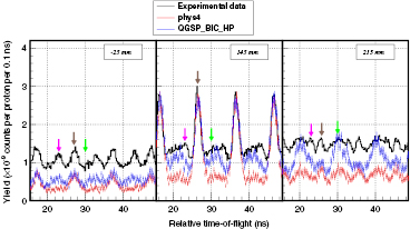
Figure 4. Experimental and simulated TOF spectra for three target positions. The position zero corresponds to the target entrance and the target has a length of 200 mm. Note that the projected range of 160 MeV protons in PMMA is 152 mm. The arrows point to different TOF components. For simplicity reasons, the arrows consider only the TOF components of a single proton bunch.
Download figure:
Standard image High-resolution image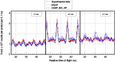
Figure 5. Experimental and simulated TOF spectra for three target positions for which the nozzle was simulated and an offset was applied to the simulated data. The offsets used were 6.2 × 10⁻¹⁰ and 3 × 10⁻¹⁰ counts per proton per 0.1 ns, respectively for phys4 and QGSP_BIC_HP. The position zero corresponds to the target entrance and the target has a length of 200 mm.
Download figure:
Standard image High-resolution imageBy analysing figure 4, it is possible to find three TOF components (indicated by arrows). The most obvious one corresponds to prompt-gamma events (brown arrow) since before and after the target this component is almost negligible but for a measurement position inside the target and the proton range it becomes prominent. Note that this component is shifting along the target since the distance travelled by protons is different for the different longitudinal positions (the TOF STOP signal is always fixed since it is defined by the cyclotron HF and only the target moves on top of the moving table). A second component is the neutron-associated events coming from the target. This component is pointed out by a green arrow in figure 4. It can be seen that this component increases along the target and it is explained by the fact that neutrons are preferably emitted forward due to momentum conservation. Finally, there is a component for which its contrast (i.e. difference between its maximum and minimum before the prompt-gamma events) and time position remain constant (magenta arrows). It was realised that the time between the prompt gammas and this component should correspond to events coming from inside the nozzle. In the sequence of such a finding, IBA provided us the full details of the nozzle in terms of geometry and materials. Note that this component is difficult to be observed in the simulations, mainly due to lower statistics.
Another remark for figure 4 is the fact that the simulated TOF spectrum baseline is lower than the experimental one. There are two possible explanations: (1) the simulations underestimate the background and (2) the geometry is not simulated with enough detail (e.g. the room was not simulated, the composition of the materials may in reality be different from those used in Geant4). Although it is reasonable to consider that the two hypotheses are playing a role, the fact that the simulated baseline is always the same relatively to the experimental one, regardless the target position, is an indication that the most critical aspect is the definition of the geometry. Henceforth this underestimation will be called room component.
In figure 5 it is possible to visualise the effect on the TOF spectra of applying a constant function to the simulated data. The results of the simulations with the nozzle description are also depicted in this figure. One can see that the TOF spectrum component is now present in the simulations, thus validating the assumption of the detection of nozzle-related events.
The finding of the room component is indeed very important since the aim of using TOF is to improve the SBR. It is of uttermost importance to have a good description of both the signal and the background or at least to be aware of the limitations of the simulations and then conclude based on that. Therefore, a constant function was applied to the simulated data used in the optimisation since it is a reasonable approach to compensate, at least partially, this effect. The room component was assumed to be linearly dependent with the detector volume and it was added to the simulated data for the optimisation.
Globally, Geant4 was able to describe the TOF spectra background shape with a reasonably good agreement for both physics lists (phys4 and QGSP_BIC_HP). However, the reference physics list showed a higher discrepancy in terms of background shape for the positions inside and after the target when comparing the relative amplitude of prompt-gamma and neutron-related TOF components. Figure 6 shows the longitudinal prompt-gamma profiles after TOF selection for the experimental data and for the cases of reference physics list and phys4. The prompt-gamma signal is overestimated in both simulated cases, although a better agreement is found for the reference physics list. Concerning the phys4 case, the disagreement is approximately 38% for the point measured at 100 mm, therefore any precision values stated herein should be addressed with some caution since they may also be overestimated. In fact, all the results presented elsewhere (Roellinghoff et al 2014) show that the precision as defined for this study is inversely proportional to the signal, hence if the signal is reduced by some factor, the same detrimental factor in the precision is expected.
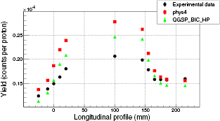
Figure 6. Experimental and simulated longitudinal prompt-gamma profiles after applying the offset to the simulated data and using a TOF window of 4 ns centred on the TOF prompt-peaks. The error bars due to the statistical error are not visible since they are within the markers. The position zero corresponds to the target entrance and the target has a length of 200 mm.
Download figure:
Standard image High-resolution imageDespite the better agreement regarding the signal yield for the reference physics list, phys4 shows a better description of the background shape. Since the impact of the signal on the precision is known but not the possible effect of a worse background description, phys4 was selected for use in this work. This issue is more critical if one compares TOF and non-TOF data. Even if an in-depth study of the origin of the overestimation by simulations is outside the scope of the present paper, it is reasonable to assume that the problem may be related to the Binary Cascade physics description since it is the critical change concerning hadronic physics between the QGSP_BIC_HP and phys4 for this energy range.
3.2. Monte Carlo data analysis
Figure 7 depicts the behaviour of the precision for each geometrical parameter.
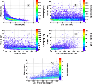
Figure 7. Precision versus a single geometrical parameter: (a) slit width, (b) slab width, (c) thickness, (d) distance from beam axis to collimator front face and (e) distance from beam axis to detector front face. Each entry is normalised to the histogram binning.
Download figure:
Standard image High-resolution imageAlthough the results shown in figure 7 can be used to verify some possible trends, each plot shows only how the precision changes for a single parameter. It is reasonable to assume that a combination of parameters may also play a role in the precision behaviour. Hence, figure 8 depicts some other design parameters that feature a combination of single geometrical parameters.

Figure 8. Properties of the camera design and their relation with precision: (a) FOV, (b) collimator pitch, (c) collimator weight per centimetre height, and (d) collimator fill factor. All these parameters except the collimator weight were defined in equations (1)–(3). Each entry is normalised to the histogram binning.
Download figure:
Standard image High-resolution imageTable 6 presents several camera configurations following three different cases (endpoints). The next list describes each case considered.
Table 6. Several camera configurations based on different endpoints. Concerning the precision values, the statistical uncertainty for one sigma is presented inside brackets.
| Case | Precision fall-off | Precision entrance | Precision profile length | FOV | Slit | Slab | Thickness | Distance axis-collimator | Distance axis-detector |
|---|---|---|---|---|---|---|---|---|---|
| 1 | 0.59(0.06) | 0.66(0.09) | 0.88(0.11) | 23.6 | 5.4 | 2.6 | 180.2 | 303.7 | 485.3 |
| 2 | –same as case 1– | ||||||||
| 3 | 0.70(0.08) | 0.87(0.12) | 1.12(0.14) | 13.1 | 3.0 | 2.1 | 190.9 | 322.3 | 516.5 |
Case 1: best precision on the fall-off position
Case 2: best precision on the profile length
Case 3: best precision on the fall-off position with a FOV lower than 15 mm
Figure 9 depicts the simulated longitudinal prompt-gamma profiles from the two geometries presented in table 6. In order to better understand the shape of the profiles, each one was divided in a stack of two components according to the particles exiting the target: the detected events due to photons and the neutron-related events.

Figure 9. Prompt-gamma profiles from the configurations presented in table 6, respectively (a) and (c) cases 1 and 2, and (b) and (d) case 3. The top profiles are separated into photons and neutron-induced events and correspond to the maximum simulated statistics (4 × 10⁹ protons). The distinction between types of events considers the particle exiting the target. The bottom profiles use a clinically-relevant amount of incident protons (1 × 10⁸ protons) as already discussed in section 2.3 and the error bars shown are for one standard deviation. The precision obtained for this statistic is 1.30 ± 0.18 mm and 1.66 ± 0.23 mm, respectively for the cases depicted in (c) and (d). The bin size is equal to the collimator pitch. The dashed line represents the proton projected range in the PMMA target.
Download figure:
Standard image High-resolution image3.3. Multivariate regression analysis
After selecting the best parametrisation following the method detailed in section 2.4, a cluster analysis was carried out on the Monte Carlo data. The clustering served as a method to select geometries to be tested against the parametrisation. The minimum number of clusters considered was three and the maximum ten. The silhouette method always yielded three clusters with the highest silhouette value. Hence, a three-cluster approach was followed for the input data. Table 7 presents the three centroids found. Around each centroid several Geant4 simulations were performed for which only one geometrical parameter was changed. Figure 10 shows the result of such a benchmarking.

Figure 10. Precision values obtained using the parametrisation and corresponding to the variation of a single geometrical parameter while keeping the others constant: varying (a) slit width, (b) slab width, (c) thickness, (d) distance from beam axis to collimator front face and (e) distance from beam axis to detector front face. Geant4 simulations are also plotted. The curve coming from the parametrisation is only plotted for the combination of geometrical parameters for which it was trained.
Download figure:
Standard image High-resolution imageTable 7. Centroids retrieved after clustering.
| Slit | Slab | Thickness | Distance axis-collimator | Distance axis-detector | |
|---|---|---|---|---|---|
| Centroid cluster 1 | 3.22 | 2.11 | 170.5 | 421.2 | 813.3 |
| Centroid cluster 2 | 3.55 | 5.49 | 155.6 | 377.2 | 723.9 |
| Centroid cluster 3 | 2.32 | 2.60 | 112.2 | 384.6 | 646.8 |
4. Discussion
The present work followed three main stages: (1) comparison of Geant4 simulations with experimental data and (2) camera design study for online monitoring in proton therapy based on Geant4 simulations, and (3) parametrisation of the simulation results in order to have a fast and accurate tool that can replace the time-consuming simulations for preliminary studies (given that the camera geometrical parameters to test are inside the range considered for the parametrisation training, otherwise all simulations must be done).
The dimensions of the camera considered for optimisation should also be carefully examined. The camera for optimisation in this paper has a height of 10 cm, but most likely a final device will be higher, thus increasing the amount of signal detected. On the other hand, the number of protons per spot considered in this optimisation may be considered as large, even for a distal one. Ultimately, these questions may only be answered with e.g. the study of several treatment plans to verify what is a reasonable spot dose to monitor and to have a camera with dimensions matching that requirement.
Due to the complex nature of the problem addressed in this work, Monte Carlo simulations were used to find a set of camera geometries able to provide millimetric precision. Table 6 presents the geometrical parameters that allow for yielding two complementary solutions: one aiming to obtain the best precision and another considering the best precision achievable with a FOV lower than 15 mm. Although FOV is not directly spatial resolution, it should have a similar tendency.
Another goal proposed in this study was to obtain meaningful information about the geometrical parameter trends driving the precision. It can be observed in figure 7 that thicker collimators seem to slightly favour better precisions. However, the geometrical parameters that influence the precision the most are the slit width and the distances from the beam axis to the collimator and to the detector. For those three parameters, the precision is improved by changing them towards a higher camera efficiency, thus making it the most important camera characteristic driving the precision. In any case, such a finding must be treated with reservation since increasing the slit width will inevitably worsen the expected spatial resolution with an as yet unpredictable impact in face of heterogeneities or ion range shifts due to unexpected morphological changes near the end of the ion path. Moreover, the ability to position the camera closer to the patient is limited by the treatment being considered (e.g. a head versus a prostate treatment), by the treatment room configuration and by the TOF-capabilities from both detectors and signal processing modules. In addition, a higher background is expected as the distance between the patient and the camera decreases. In order to fully address these issues, further experimental work with a full-size prototype is needed. Figure 10 also supports these findings, except for the case of the distance from the beam axis to the collimator, where no significant variation is observed. It is not clear why, but it is reasonable to assume that the starting points (i.e. the centroids) for the parametrisation testing were in a stable region for this parameter.
Figure 8 provides further insights regarding the trends in the geometrical parameters. The most striking information comes from the quantities that correlate slab and slit widths (i.e. collimator pitch and fill factor). While the slab width alone does not produce an observable effect on the precision, it can be seen that the best precision values are obtained for a collimator pitch between 6 mm and 8 mm, and for fill factors between 0.3 mm and 0.6 mm. An important and interesting remark is that the camera design that corresponds to the best precision has a collimator pitch and a fill factor of 8 mm and 0.325, respectively. Furthermore, a high collimator fill factor (>0.7) shows a strong detrimental effect on the precision. Concerning FOV, the trend is to have better precisions with a better camera efficiency, while the collimator weight does not have an obvious impact on the precision, except for very light (<2 kg cm−1) and very heavy (>7 kg cm−1) collimators for which the precision is generally worse.
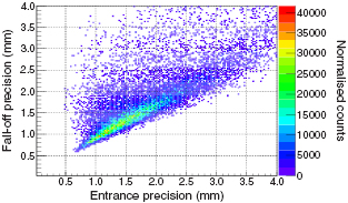
Although most of the discussion is centred on the precision in finding the prompt-gamma fall-off position, the precision in the retrieval of the entrance position is also of utmost importance. The device being developed aims at registering all events along the ion path, thereby providing a full prompt-gamma profile. With such a profile it is possible to retrieve the ion range by making use of both the entrance and the fall-off positions. Due to the lower number of events at the entrance (see the profiles shown in figure 9) a worse precision is expected for this position. Figure 11 supports this claim since it shows that the precision for the entrance position is systematically worse than the one for the fall-off for the simulated geometries.
Figure 11. Entrance and fall-off precisions from the simulated camera geometries. Each entry is normalised to the histogram binning.
Download figure:
Standard image High-resolution image
However, the measurement of the entrance position by means of prompt gammas may not be mandatory. It can be retrieved with e.g. the data provided by an optical surface imaging system intersected with the information of the beam position coming from the treatment planning system (TPS). The optical system provides information that is independent of the statistics (i.e. spot size) with a relatively good precision. For example, (Schöffel et al 2007) found an accuracy of 1.02 ± 0.51 mm (with a maximum deviation of 2.86 mm) on retrieving the thorax surface of healthy volunteers for a commercially-available system (accuracy estimated considering the deviations between volunteer displacements and recommended couch transformations calculated by a 4 degrees-of-freedom registration using the optical system). On the other hand, a full prompt-gamma profile can potentially attain a better precision for the entrance position (see table 6, but notice that those results are from Geant4 simulations considering a homogeneous target with a very well defined target entrance) and the entire measurement is made with a single device. Additionally, it was suggested elsewhere (Bom et al 2012) that the prediction of off-beam deviations is prone to failure if only the prompt-gamma fall-off position is known, while having more information about the prompt-gamma profile can help overcome such a limitation by using registered correlation (Gueth et al 2013). In any case, the precision on the retrieval of a given position with this camera intrinsically depends on the spot statistics.
Concerning the parametrisation, figure 10 shows an overall good agreement between parametrisation and Monte Carlo simulations. The final result is an analytical tool based on Monte Carlo simulations that can assist on further developments of the camera in situations where one must deal with mechanical constraints like having the exact dimensions of the slabs from a supplier or in the positioning of the camera inside the treatment room. The striking advantage of this tool is to possess the capacity to roughly estimate the precision for different geometries very rapidly. However, the clear disadvantage is the inability to accurately predict the precision for sets of geometries that were almost absent during the training.
Although this study is focused on proton therapy monitoring, it is important to note that all the procedures followed in this work should also be applicable to other ion species, namely carbon ions. However, care must be taken since the proposed solutions herein should not be directly usable in different treatment scenarios. For example, a higher background in a carbon ion irradiation is expected, thus it is reasonable to presume that the camera should be placed in a more distant position in respect to the beam axis in order to benefit from a better separation of signal and background components in TOF spectra.
5. Conclusions
Herein is presented a study to provide a set of multi-slit collimated cameras optimised for hadrontherapy online monitoring using prompt gammas. The initial step consisted of a comprehensive review of different physics lists of Geant4 for selecting the ones with the best outcome. The comparison of the results obtained with these physics lists with experimental data from single-slit experiments with proton irradiations assisted us in choosing the most accurate set of physics models among the ones tested. It also allowed for adding a correction factor to the data to take into consideration the treatment room environment. Although the value found is specific for the room in which the experiment was performed, the methodology and considerations are valid for any treatment scenario.
The second step provided not only two different camera designs, but also a detailed investigation concerning the trends driving the precision of the multi-slit collimated cameras was performed. The two different camera designs proposed consider different endpoints based on the trade-off between camera detection efficiency and spatial resolution.
Finally, the development of an analytical tool able to predict the precision for any given camera geometry was described.
Acknowledgments
We would like to acknowledge IBA for providing the nozzle details of the system installed at the clinical facility WPE, Essen and for hosting the experiment there.
The present work was performed in the framework of FP7-ENTERVISION network (Grant Agreement number 264552), FP7-ENVISION programme (Grant Agreement number 241851), LabEx PRIMES ANR-11-LABX-0063/ANR-11-IDEX-0007, France HADRON, and ETOILE's research programme (PRRH) at Université Claude Bernard Lyon 1 (UCBL).
We also gratefully acknowledge IN2P3 Computing Center (CNRS) for providing a significant amount of the computing resources and services needed for this work.