

Abstract
Ion beam therapy promises enhanced tumour coverage compared to conventional radiotherapy, but particle range uncertainties significantly blunt the achievable precision. Experimental tools for range verification in real-time are not yet available in clinical routine. The prompt gamma ray timing method has been recently proposed as an alternative to collimated imaging systems. The detection times of prompt gamma rays encode essential information about the depth-dose profile thanks to the measurable transit time of ions through matter. In a collaboration between OncoRay, Helmholtz-Zentrum Dresden-Rossendorf and IBA, the first test at a clinical proton accelerator (Westdeutsches Protonentherapiezentrum Essen, Germany) with several detectors and phantoms is performed. The robustness of the method against background and stability of the beam bunch time profile is explored, and the bunch time spread is characterized for different proton energies. For a beam spot with a hundred million protons and a single detector, range differences of 5 mm in defined heterogeneous targets are identified by numerical comparison of the spectrum shape. For higher statistics, range shifts down to 2 mm are detectable. A proton bunch monitor, higher detector throughput and quantitative range retrieval are the upcoming steps towards a clinically applicable prototype. In conclusion, the experimental results highlight the prospects of this straightforward verification method at a clinical pencil beam and settle this novel approach as a promising alternative in the field of in vivo dosimetry.
Export citation and abstract BibTeX RIS
1. Introduction
Accelerated charged particles such as protons have been proposed for cancer treatment since 1946 (Wilson 1946). These particles stop at a well defined depth (the particle range), where the ionization density reaches its maximum (the Bragg-peak) and falls sharply behind it. In theory, the dose can be focused on the tumour and the damage to healthy tissue is minimized compared to photon therapy.
Conversely, ion beam therapy is a more expensive (Goitein and Jermann 2003) and less mature irradiation technique. Is there enough evidence of clinical superiority (Freeman 2012) to justify its high costs? This controversy (Orton and Hendee 2008), chapters 2.11–2.13, arisen in the medical community spins strongly around the intrinsic range uncertainties (Deasy 1994).
In contrast to photon therapy, patient positioning, organ motion, minor density and anatomical changes during or between treatment fractions, stopping power uncertainties, among other factors (Andreo 2009, Grün et al 2013), are prone to yield high dose deviations with respect to the original treatment plan.
In the scientific community, diverse methods have been proposed during the last decades for in vivo particle range assessment (Knopf and Lomax 2013), but are not yet at the stage of widespread application in clinical routine. One approach is the measurement of the spatial distribution of the prompt gamma rays produced in nuclear reactions between the projectile ions and nuclei of the irradiated tissue. The prompt gamma rays are emitted promptly, exit the patient without severe attenuation and their emission distribution is closely correlated with the dose deposition map of the incident ions, as shown experimentally by Min et al (2006). Such correlation is dependent on prompt gamma energy and tissue composition (Moteabbed et al 2011, Gueth et al 2013, Polf et al 2013, Janssen et al 2014).
In the recent years, there is a trend towards systems with less expensive hardware and, probably, faster translation into clinical practice (Testa et al 2014, Assmann et al 2015). In this context, at OncoRay and Helmholtz-Zentrum Dresden-Rossendorf (HZDR), an innovative method for range assessment complementary to the actively and passively collimated prompt gamma ray imaging systems has been proposed (Golnik et al 2014): the prompt gamma ray timing (PGT). Based on the measurable transit time of ions through matter, the detection times of prompt gamma rays encode essential information about the depth-dose profile. Hence, a single detector in a timing spectroscopy setup aims to verify the range at minimum expense and without collimation, just measuring the time between particle entrance in the target and reception of the prompt gamma. As usual, the accelerator radio frequency can be used as time reference.
The proof of principle experiment carried out at a research accelerator (Golnik et al 2014) raises expectations about the future of the PGT method. To evaluate its potentials as well as its limitations, a dedicated experiment at a clinical therapy facility with heterogeneous targets and a pencil beam is mandatory.
The aim of this paper is:
- To test the robustness of PGT at a clinical proton accelerator against background and bunch time stability, and examine the factors limiting its applicability and precision.
- To characterize the bunch time structure of the proton beam and its dependence on the energy.
- To analyse if the PGT method is able to detect range variations due to the presence of heterogeneities.
- To estimate the precision of the retrievable range differences as a function of the collected statistics.
- To assess the mandatory next steps for translation into clinical practice.
Altogether, this work aims at exploring the problems and weak points that may arise when a technique proven at a research accelerator is translated into a real medical scenario, and proposes some strategies to circumvent or solve the encountered limitations. In other words, we do not intend to present a final clinically applicable prototype, but rather investigate and mark the way towards it.
2. Materials
2.1. Detectors
Three monolithic scintillation detectors are used to compare the PGT spectra at different geometries, as well as to check the robustness and compliance of the method. The experimental data are acquired in parallel for all detectors. Their characteristics are summarized in table 1.
Table 1. Monolithic scintillation detectors available in the experiment.
| Alias | Material | ⌀  Length Length |
PMT model | Rise time / ns | Rationale |
|---|---|---|---|---|---|
| B1 | BaF2 | ![$\left[25:38\right]\times 30$](https://content.cld.iop.org/journals/0031-9155/60/16/6247/revision1/pmb515768ieqn002.gif) mm mm |
R2059 |  |
Time resolution |
| B3 | BaF2 |  mm mm |
R2059 |  |
Time resolution |
| L0 | LaBr3:Ce |  |
R2083 |  |
Energy resolution |
Note: B3 and L0 are cylindrical, whereas B1 is a tapered cone (for optimum time resolution). All PMTs are from Hamamatsu. The rise time refers to the anode signal.
2.2. Electronics
Each scintillation crystal is optically coupled to a Photomultiplier tube (PMT), whose type is given in table 1. The modular electronics employed in this experiment are similar to those described in Hueso-González et al (2014). For the B1 and B3 detectors, the anode signal is fed to a constant fraction discriminator (CFD) for trigger generation, while the dynode signal is shaped and fed to a peak-sensing analog to digital converter (ADC). For the L0 detector, the anode signal is amplified and split. One branch is for the CFD, the other for a charge to digital converter (QDC). A time to digital converter (TDC) monitors the output of the CFD. The energy deposit in the crystal is measured by the QDC or ADC, whereas the gamma interaction time is given by the TDC module.
2.3. Accelerators
For the verification of the PGT method, we conduct an experiment at the Westdeutsches Protonentherapiezentrum Essen (WPE), Germany, a clinical proton therapy facility comprising a Cyclone 230 (C230) isochronous cyclotron of IBA (Louvain-la-Neuve, Belgium). Complementarily, the detector time resolution is characterized at the Electron Linac for beams with high Brilliance and low Emittance (ELBE) facility at HZDR using the same detector set and electronics. The methodology developed for such analysis is published in Hueso-González et al (2014).
2.3.1. Setup at WPE proton accelerator.
The experiment is carried out in the gantry treatment room TR4 with a single incidence angle (horizontal) pencil beam (no scanning) and manual control mode. The patient table is aligned to the gantry room isocenter. A target holder mounted on a linear stage with remote control is placed on the patient table, see figure 1 (bottom).

Figure 1. Top: schematic sketch of the experimental setup at the WPE proton therapy facility and of the longitudinal cross section of the target. The accelerated protons bunched with 105.98 MHz (corresponding to 9.436 ns separation) collide with the target. As a result of nuclear reactions between the protons and nuclei of the phantom, prompt gamma rays are emitted and measured with a monolithic scintillation detector. The PMMA cylindrical target contains a cavity or bone insert of thickness t located at a distance z from the beam entrance point. Bottom: photograph of the experimental setup with three detectors at different ring angles  . The linear stage on the center of the ring holds the two hollow joined half cylinders, in which PMMA, cavity or bone slices can be inserted. The beam incidence is horizontal from the left, where the snout of the nozzle is seen.
Download figure:
Standard image High-resolution imageProtons bunched with  MHz are shot onto a target with an energy adjustable between 70 and 230 MeV. Two hollow polymethyl methacrylate (PMMA) half cylinders with an external diameter of 15 cm, an internal of 5 cm, a length of 20 cm and a density of
  g cm
g cm are available. Cylindrical slices of 5 cm diameter and different thicknesses can be inserted into the hollow cavity left inside the two joined half cylinders. Available slice materials are PMMA, bone-equivalent tissue or air (hollow slice). Custom target configurations can thus be constructed by joining slices heterogeneously. The enclosing half cylinders are used to reproduce the therapeutic irradiation conditions concerning neutron production and moderation in surrounding tissue. The spatial dimensions are measured with 0.2 mm precision.
The bone-equivalent material corresponds to SB3 cortical bone, model 450 from Gammex-RMI (Middleton, USA). The measured density is  g cm
g cm . The electron density, effective atomic number and elemental composition are listed in (Helmbrecht 2015, appendix A).
Various detectors are arranged at the desired angle and distance as described in figure 1 (top) to measure the prompt gamma rays exiting from the target. A photograph of the experimental setup is shown in figure 1 (bottom). For a given proton energy, we label a homogeneous target as full target if the protons are stopped completely inside it.
The positioning inside the gantry room is based on the built-in laser room system and the pencil beam spot size is measured with an EBT3 gafchromic film from International Specialty Products (Wayne, New Jersey) placed on the front face of the target (from beam point of view). The position of the target with respect to the gantry room isocenter is described in section 3.4.
3. Methods
3.1. Detector and module settings
We choose detectors and electronics' settings according to the energy range of prompt gamma rays that are correlated to the particle range (Verburg et al 2013), namely higher than 1 MeV and lower than 8 MeV. We adjust the detector voltage so that the height of the CFD input signal lies around 150 mV when  Co source photons (1.173 and 1.333 MeV) are detected. The CFD threshold is then set to 1.0 MeV. The zero-crossing is adjusted empirically with a
  Co source by optimizing the coincidence resolving time (CRT) with respect to B1 (the reference).
With the same detectors and electronics, we perform an experiment at ELBE in a setup similar to Hueso-González et al (2014). The goal is to accurately measure the intrinsic detector time resolution and time walk, and apply a time slewing correction retrospectively to the data acquired at WPE.
3.2. Proton bunch phase stability
The PGT method is based on the dependence of the prompt gamma ray emission time (or ion transit time) on the particle depth of interaction. As the protons are bunched with the accelerator RF, it can be used as a time reference for the beam entrance in the target (clock start) if the beam parameters remain stable.
This methodology, a standard in time-of-flight measurements, is successfully applied by Golnik et al (2014) for testing the PGT method with a fixed proton energy at a research accelerator. However, one has to wonder if this technique is also robust and stable on a longer term at a clinical accelerator.
In any cyclotron, the charged particles are accelerated by a high voltage alternating with the so called radio frequency (RF). This frequency must be a multiple of the particles' orbital frequency in the isochronous electromagnetic field. If this condition is not kept completely stable (Schutte 1973), the bunches may still be accelerated but not in perfect resonance. This would lead to phase shifts between RF signal and extracted beam bunches, i.e. the PGT spectrum would displace.
To analyse this potential effect in the clinical isochronous cyclotron of IBA, we perform the following experiments in a setup similar to figure 1 (top) with a homogeneous PMMA target at a fixed proton energy:
- (i)We acquire short PGT spectra of similar statistics separated from each other about one hour. The comparison of the, in principle, equivalent spectra can shed light on potential long-term instabilities of the bunch phase relative to the RF.
- (ii)We measure PGT spectra for several (very close) values of the main coil current of the cyclotron. Corresponding variations of the magnetic field change the orbital frequency of the accelerated ions, which is expected to affect (at each turn) the phase slip of particle bunches during acceleration and thus their time correlation at the extraction radius relative to the RF. Potential relative shifts in the time axis of the corresponding PGT spectra will quantify the effect of small instabilities of the magnetic field or the accelerator RF, which might be caused by thermal effects (among others).
3.3. Proton bunch time structure
The beam bunch time structure is a key parameter for the accuracy of the PGT method. Whereas the detector time resolution can be reduced down to 150 ps full width at half maximum (FWHM) with fast scintillation detectors (see section 4.1), experiments with a slit gamma camera at clinical accelerators show a prompt gamma width between 1.2 and 2.8 ns FWHM (Verburg et al 2013). This suggests that a significant contribution to the global system time resolution is the proton bunch time spread.
Such spread is dependent on the proton energy for the C230, as a graphite or beryllium degrader brakes the protons from 230 MeV down to the desired energy. That introduces an additional energy straggling (Clasie et al 2012) and thus a velocity spread, which also leads to a time spread depending on the length of the beam line. Indeed, we perform our experiments in TR4, the farthest treatment room from the cyclotron, which implies the worst case bunch spread. Therefore, the conclusions of this paper regarding the applicability and robustness of the PGT method are implicitly valid for the remaining rooms.
To characterize the intrinsic bunch time spread (namely at 230 MeV, where the thick degrader is replaced by an aluminium foil), we perform a measurement with a detector in downstream orientation, see figure 1 (top), and a thin PMMA target. Note that, for full targets, the contribution of the proton transit time to the width of the PGT peak has the same order of magnitude as the proton bunch spread, an effect which had been either overlooked or not explicitly discussed until (Biegun et al 2012, Robert et al 2013).
We repeat the measurement of the bunch time spread for representative energies covering (to a large extent) the range applied in therapeutic irradiations: 160 MeV and 100 MeV. These measurements characterize the effect of the degrader on the time spread. In addition, for the 100 MeV case, we analyse a potential reduction of the bunch time spread by changing the settings of the energy selection system. Namely, we close the momentum slit, a handle which limits the energy spread of the beam after the degrader. With the usual clinical setting, the relative momentum spread  is
is  0.5%.
0.5%.
3.4. Systematic measurement program
A systematic measurement program is accomplished for three energies of interest: 100, 160 and 230 MeV. Although the latter is a rather infrequent energy in clinical practice, it has an important research interest as the bunch time spread is expected to be the lowest and, hence, the upper limit for the precision of the PGT method can be explored.
The nominal energy precision is 0.7 MeV, so that the error in the range in water is below 1.2 mm (Clasie et al 2012). For the sake of clarity, we refer always to proton energies at the exit of the energy selection system. The actual energy at the target's front face is lower due to losses in the nozzle and beam exit window:  ,
,  and
and  MeV for a respective initial proton energy of 100, 160 and 230 MeV. The corresponding proton range in a full PMMA target is
  ,
,  and
and  cm.
cm.
Three detectors are measured in parallel (individual trigger on each of them). The geometrical arrangement is depicted in figure 1 (bottom), with B1 and L0 in upstream orientation ( ,
,  ) and B3 placed downstream (
 ).
).
The reference full PMMA target is aligned with 1 mm precision on the linear stage so that, for a given proton energy, half of the particle range lies on the ring center on which the detectors are rotated. This way, the emission distribution is in the middle of the field of view of the detectors. The center of the ring is  cm downstream from the gantry room isocenter, i.e. to the right in the beam axis as depicted in figure 1. Note that d and
  are measured with respect to the ring center, not the room isocenter.
For each proton energy, we perform the following measurement series with the hollow PMMA cylinder and its customizable insertions:
- Stacked target. Slices of PMMA are taken out of the full target, so that the protons are not completely stopped inside it. The slices are removed from the back face of the target.
- Air cavities. Air cavities with a thickness t of 2, 5 and 10 mm are inserted at different positions z, as described in figure 1.
- Bone inserts. A slice of bone-equivalent material with a thickness t of 20 mm is placed at different positions z.
Another possible experiment, namely the variation of the range by increasing the beam energy in small steps, is discarded because the relative time offset of the PGT profiles and the bunch time structure are dependent on the beam energy.
Despite a careful alignment with the room laser system, the spatial accuracy in the target front face position between measurements is estimated to be about 1 mm (statistical), as the upper half cylinder has to be temporarily removed each time a slice is replaced. The error of the detector distance d is 2 mm (systematic), but does not vary between measurements. The angle precision is  (systematic). The protons impinge the target approximately at the center of the target: this position is verified with two gafchromic film at the target front and back face with 3 mm precision (systematic).
The systematic errors may introduce a constant global offset in all PGT spectra, which has however little importance when comparing PGT measurements with respect to a reference one. Rather, the statistical error of the front face position has a significant influence, as it may shift the leading edge of PGT spectra of consecutive measurements. For example, the theoretical time jitter in the PGT spectrum (due to a target positioning error) of a detector at  and
and  cm for 100 MeV protons is
  10.4 ps mm
 , according to the additional proton time of flight
  7.8 ps mm
 and extra gamma time of flight
  2.6 ps mm
 .
.
3.5. Data acquisition rate
The duration of each measurement of the systematic program described above is around 6 min with a cyclotron current between 10 and 100 pA. The reason for choosing a current far below the clinical current (between 1 and 3 nA) is that the data acquisition with the current electronics sustains a maximum throughput of 40 kcps. The detector distance d to the ring center is adjusted between 20 cm and 60 cm so that, for a given beam current and proton energy, the individual detector trigger rate (above 1 MeV) is  30 kcps and the system dead time is 50% at most.
This experiment is not intended to explore the throughput capabilities neither to provide clinically applicable PGT prototypes, but to acquire spectra in a clinical scenario with enough statistics despite long measurement times and low beam current: around  irradiated protons per measurement, which translate to at least
  valid gamma events per detector (entries in the PGT histogram). Depending on the detector considered, we acquire between
  and
and  gamma events per proton.
3.6. Data analysis
All the time spectra are corrected according to the time slewing characterization carried out at the ELBE experiment, see details in Hueso-González et al (2014).
The PGT spectra are analysed for two different gamma energy filters: between 1 MeV and 6.5 MeV (gaining statistics due to multiple characteristic gamma lines), and between 3 MeV to 5 MeV (matching with the pronounced 4.4 MeV line and the corresponding escape peaks). In the figure captions, for compactness, we will refer to these filters as energy threshold of 1 and 3 MeV, respectively. Please note that, in all experimental spectra, the energy scale does not refer to the incident gamma energy but to the energy deposit in the detector.
In the offline analysis, before overlaying them, the spectra are normalized according to annotated proton charge (from a built-in ionization chamber used in clinical routine) and system dead time correction. We do not intend an absolute normalization, but rather a relative one between PGT measurements. Therefore, we label the vertical axis of our histograms as Counts without magnitudes. In all PGT spectra, the bin width is 24.41 ps.
Due to the high dynamic system dead time in our VERSAModule Eurocard (VME) electronics and parallel operation of several detectors in the same crate, the estimation of the dead time correction factor by the scaler in our electronics is not very accurate: the precision of the (relative) normalization is not expected to be better than 5% between consecutive measurements.
In some cases, one can correct by eye normalization fluctuations or phase drifts according to the expected leading edge or maximum value of the PGT spectra. The rationale is to at least compare them qualitatively and illustrate the effect of a stacked target measurement or the presence of heterogeneities. Nevertheless, the quantitative analysis can only be justified with more reliable and accurate measurement tools in upcoming experiments. If present, the illustrative manual correction of normalization and bunch phase drift will be stated clearly in the figure captions.
3.7. Modelling of PGT spectra
The PGT spectra encode information about the prompt gamma spatial emission distribution. However, neither the conversion of time to space profile nor the direct quantitative retrieval of the range are trivial procedures. One approach is to compare the measured PGT spectrum with a simulated one once a spatial emission profile is known. The profile, which depends on tissue composition and reaction processes involved (gamma lines), can be obtained by a Monte Carlo (MC) simulation (Verburg et al 2012), although discrepancies between different codes and experimental validation need still to be addressed (Schumann et al 2015). A precise modelling must also incorporate the detector response (detection probability and pulse height distribution for a given gamma energy) and the selected energy window. However, this is out of the scope of this work and will be dealt in forthcoming papers.
It turned out that our experimental results, obtained with rather simple target configurations, are well described with a coarse approximation of the prompt gamma emission distribution: the simBox model (Golnik et al 2014). It assumes, for simplicity, a flat spatial emission profile (with a scale factor depending on the material), correlates the interaction depth with the gamma emission time based on stopping power data, accounts for the gamma time of flight to the detector and convolves the timing profile with the system time resolution. This model is extended within this study in order to include the detector sensitivity and attenuation of prompt gammas inside the target.
It should be emphasized that the simBox model is just a transitory tool in the roadmap towards clinical application. The effect of having an oversimplified flat spatial emission profile can surely lead to differences between measurement and model at the falling edge (near the Bragg peak), specially for detectors in downstream direction, whose covered solid angle is maximum for this region of the depth profile. For this reason, the simBox model will only be used in the current paper for upstream detectors. We want to investigate if range deviations of few millimetres can be seen based on changes of the timing spectra, and compare if these shifts follow the expected trend and are in qualitative agreement with the model. This strategy can give already some hints that mark the way towards quantitative range retrieval, notwithstanding the need of more reliable models, which are considered a further indispensable step.
4. Results
4.1. Intrinsic detector time resolution
Table 2 summarizes the energy resolution and coincidence resolving time (CRT) of all detectors as measured with a  Co source.
Table 2. Detector energy resolution and CRT for photons of a  Co source.
| Alias | Energy resolution | CRT versus B1 |
|---|---|---|
| B1 |  % % |
Reference |
| B3 | / |  ps ps |
| L0 |  % % |
 ps ps |
Note: The energy resolution (FWHM) is measured at the 1.173 MeV photopeak. The time resolution (FWHM) is measured always with respect to the B1 detector and an individual CFD threshold of 1.0 MeV.
At the ELBE accelerator, the result of the intrinsic detector time resolution as a function of the photon energy is shown in figure 2. The electronic resolution (precision of the time stamp) with which the ELBE RF is measured,  ps FWHM, is already subtracted.

Figure 2. Intrinsic time resolution (FWHM) of the detectors measured at the ELBE bremsstrahlung beam as a function of the energy deposit. CFD threshold level corresponds to about 1.0 MeV energy deposit. The electronic resolution of the RF, i.e. the precision of the time reference, is already subtracted.
Download figure:
Standard image High-resolution image4.2. Illustrative energy over time spectra
Figure 3 shows three illustrative cases of energy over time spectra for 230 MeV protons. In (a), corresponding to an upstream detector, we can distinguish clear prompt gamma lines corresponding to 6.1 MeV and 4.4 MeV, as well as single and double escape peaks. In addition, we can identify the time uncorrelated gamma line of neutron captures on hydrogen at 2.2 MeV (horizontal line). Conversely, (b) evinces a more compressed PGT distribution, no energy-resolved gamma lines (B3 has worse energy resolution) as well as a considerable increase of background. The bump located at (4 to 6 ns; 1 to 4 MeV) may be related to fast neutrons (secondary gammas), whereas the vertical structure at ( 7 ns; 3 to 8 MeV) could be associated with scattered protons leaving the target. (c) corresponds to a thin PMMA target, and vertical structures due to scattered particles are also visible.
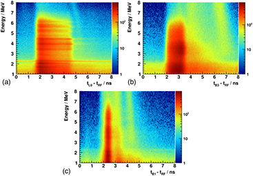
Figure 3. (a) Energy over time spectrum of the L0 detector at  ,
,  cm and a homogeneous full PMMA phantom. (b) Analogous spectrum for the B3 detector at
  ,
,  cm. (c) Spectrum of the B1 detector at
  ,
,  cm with a thin PMMA target. In all cases, the proton energy is 230 MeV and the color scale refers to the number of collected counts.
Download figure:
Standard image High-resolution imageThe reason for the compressed PGT profile is the angle  : for downstream detectors, the protons and gammas fly both downwards, and the gamma time of flight to the detector for the entrance point is larger than for the stopping point. This reduces the spread of arrival times at the detector. On the contrary, for upstream detectors, the gammas travel backwards, in opposite direction to the protons. The gamma time of flight is larger at the stopping point than at the entrance point, and the emission time spectrum is stretched. For
  and large d, all gamma rays need the same time of flight to the detector, and the PGT spectrum reflects just the emission time distribution.
4.3. Proton bunch phase stability
The PGT spectra shown in figure 4 (left) correspond to independent measurements with the B3 detector at  for 230 MeV protons impinging a full homogeneous PMMA target. The mean value of the depicted distributions is shown in figure 4 (right).

Figure 4. Left: PGT spectra of the B3 detector at  ,
,  cm, a homogeneous PMMA target and a proton energy of 230 MeV. Independent redundant measurements of about 5 min with a separation of around 1 h are overlaid. Spectra are normalized to the number of protons (obtained from the measured charge and considering the system dead time correction). Energy threshold is 1 MeV. Right: mean value
  of the PGT distributions. The green arrow illustrates the PGT effect corresponding to a 1 cm target shift.
Download figure:
Standard image High-resolution imageThere is an evident drift of the PGT spectrum at a scale of hours: the mean value shifts around 400 ps in a time span of four hours. Albeit a constant target position and proton energy, the PGT spectrum is not stable. The origin of this deviation is attributed to the phase shift of the proton bunch with respect to the RF signal.
The results of the complementary experiment to analyse the stability of the bunch phase with respect to the RF when slightly varying the cyclotron main coil current are shown in figure 5 (left). The dependence of the distribution's mean value on the magnet current is plotted in figure 5 (right) and is more or less linear in this range.
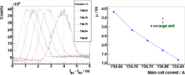
Figure 5. Left: PGT spectra of the B3 detector at  ,
,  cm, a full homogeneous PMMA target and a proton energy of 160 MeV for different values of the main coil current of the cyclotron (detailed in the legend). Spectra are normalized to their respective maximum. Energy threshold is 1 MeV. Right: mean value
  (Gaussian fit with linear background) of the PGT distributions. The green arrow illustrates the PGT effect corresponding to a 5 cm target shift. The blue dashed line is just a subsidiary line connecting the points.
Download figure:
Standard image High-resolution imageA shift in the time distribution of about 14 ps mA at an average current of
  740 A is measured. This reflects the extremely high sensitivity of the PGT spectrum mean value to cyclotron instabilities: relative current variations of one per million result in measurable center of gravity shifts and thus affect or limit the long-term precision of the PGT method if no bunch phase monitor is deployed.
4.4. Proton bunch time structure
In figure 6 (left), the dependence of the bunch width on the proton energy is demonstrated indirectly when measuring the prompt gamma rays produced in a thin PMMA target.
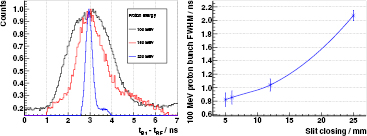
Figure 6. Left: PGT spectra of the B1 detector at  ,
,  cm,
cm,  cm, with a thin PMMA target (
 cm) for three different proton energies and the usual slit closing (25 mm) at the WPE gantry TR4. Spectra are normalized to their respective maximum and shifted in time to match their centroids for correcting the different proton time of flight. Energy threshold is 3 MeV. Right: proton bunch time spread (FWHM after numerical background subtraction) at 100 MeV proton energy and a full PMMA target for the B3 detector at
  ,
,  cm. Gamma energy threshold is 3 MeV. Proton transit time as well as RF and detector time resolution are already subtracted.
Download figure:
Standard image High-resolution imageThe presence of a tail right from the main peak in the spectra is related to secondary charged particles, mainly scattered protons, as the thin target does not stop them completely and can thus generate delayed but correlated background (see figure 3(c)). This is not suppressed even though we increase the gamma energy threshold to 3 MeV for figure 6 (statistics are not critical in this case). The bunch spread is measured with different detectors and detailed in table 3 by determining the FWHM of the PGT distributions and subtracting the proton transit time as well as the intrinsic detector and RF time resolution.
Table 3. Proton bunch time spread (FWHM) at the gantry TR4 of the WPE accelerator for different detectors ( ,
,  cm,
cm,  cm,
cm,  ,
,  cm,
cm,  cm,
cm,  ,
,  cm), three proton energies and the usual slit closing (25 mm).
| Alias | 100 MeV | 160 MeV | 230 MeV |
|---|---|---|---|
| B1 |  ns ns |
 ns ns |
 ps ps |
| B3 |  ns ns |
 ns ns |
 ps ps |
| L0 |  ns ns |
 ns ns |
 ps ps |
Note: The fit is done with a prompt gamma energy threshold of 3 MeV. The proton transit time, intrinsic detector time and RF resolution are already subtracted.
Figure 6 (right) shows the resulting bunch time spread at 100 MeV for different values of the momentum slit, see section 3.3. All measurements of section 4.5 are done with a momentum slit opening of 25 mm, i.e. the usual clinical setting.
4.5. Systematic measurement program
4.5.1. 230 MeV proton energy
Stacked target. Figure 7 (left) evinces the potential of the PGT method at an energy of 230 MeV compared to 160 or 100 MeV due to the very low bunch time spread, see figure 6 (left). Individual characteristics can be identified along the spectrum shape, instead of focusing on the distribution momenta, as done in the experiment at the AGOR accelerator (Golnik et al 2014).
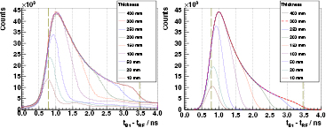
Figure 7. Left: experimental PGT spectra of the B1 detector at  ,
,  cm, for 230 MeV protons and different PMMA target thicknesses (listed in the legend). Spectra are normalized according to dead time and charge and retuned within a 5% error margin for illustrative purposes. In addition, the bunch phase shift is corrected to match all the leading edges of the spectra. Energy threshold is 1 MeV. Right: spectra calculated with the simBox model. The time offset relative to experiment is adjusted manually. Both: the two vertical dashed lines refer to the expected front face and proton range positions.
Download figure:
Standard image High-resolution imageIn the case of the full PMMA target, the proton stopping point is at 28.0 cm depth. A smooth leading edge is identified in the PGT spectrum, which is associated to the front face of the target (beam entrance point). A trailing edge related to the distal fall-off is found, but with lower relative intensity. Despite the expected increased gamma production rate within the Bragg peak, the measured profile does not reproduce it directly due to the following factors:
- Solid angle effects for upstream detectors, i.e. Bragg peak is much farther away than the entrance point.
- Larger path through PMMA (attenuation) for the prompt gammas emitted at the distal edge.
- Transformation between measured time, gamma emission time and nuclear interaction depth. As the particles' velocity is not constant, the conversion from space to time is not linear and the histogram is stretched over more time bins close to the Bragg peak (slowest protons) than at the beam entrance point (fastest).
The removal of a slice from the target's rear face links to a decrease in the area and shift to the left in the mean value of the PGT distribution over the whole thickness range studied (except for the 400 mm case). For the thinner targets (thickness  50 mm), the reduction in the area correlates with a decrease in the maximum of the curve, as the proton transit time effect has the same order of magnitude as the system time resolution. Conversely, for the thicker targets, the effect of removing a slice can be clearly identified as a decrease of the prompt gamma production at a given depth, which changes the right leaf of the distribution but not the maximum. Comparing the 300 mm and 400 mm cases, we observe no change at all. This confirms the intuitive idea that adding material beyond the particle range (280 mm) does not have any effect on the PGT profiles, as the protons are completely stopped at equal depth in both cases and the region of prompt gamma production is equivalent.
Figure 7 (right) shows the PGT distributions based on the simBox model. The general shape along the depth axis is reproduced, however, near to the right fall-off, the model fails to incorporate the rectangular edge of the 300 and 400 mm targets, in which the protons stop completely. This is related to the fact that the simBox model underestimates the gamma production rate close to the Bragg peak. Furthermore, the background is not included in the model.
Air cavities. An extensive study about air cavities of different thicknesses and locations inside the full PMMA target is accomplished for 230 MeV protons, as shown in figure 8. By comparing the PGT spectra, one can visually identify a deficit in the gamma production of a magnitude correlated to the cavity thickness at the time position corresponding to its location, as well as a shift to the right in the position of the trailing edge (overshoot). Air cavities and thus range differences down to 2 mm can be retrieved with the gathered statistics and without any sophisticated numerical analysis.
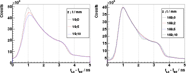
Figure 8. Experimental PGT spectra of the L0 detector at  ,
,  cm, for 230 MeV protons and different air cavities inside the full (400 mm) PMMA target at
  (position: thickness as described in figure 1). Distributions are shifted in time to match their leading edges: at 50% of the rise for right figure, at 10% for the left one as the cavities close to the target's front face affect the 50% level. Spectra of left figure are normalized to charge and dead time, for the right figure to their respective maximum. Energy threshold is 1 MeV.
Download figure:
Standard image High-resolution imageThese experimental spectra are in significant agreement with the modelled ones, if we exclude the region near the Bragg peak. The centroid of the cavity, namely the time point with the largest deficit in counts with respect to the homogeneous case, is depicted in figure 9 for different locations z of the 10 mm cavity. The values expected by the simBox model are in reasonable agreement with the experimental ones.
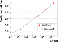
Figure 9. Measured time position (centroid of the deficit) of a 10 mm cavity at different distances z from the PMMA target's front face with the L0 detector. The experiment is compared to the values expected according to the simBox model. The relative time offset is adjusted empirically.
Download figure:
Standard image High-resolution imageBone inserts. A bone-equivalent slice of 20 mm thickness is inserted at different locations inside a PMMA target for 230 MeV protons. The PGT distributions measured with the L0 detector are shown in figure 10. The bone insert correlates evidently with an increase of the prompt gamma production with respect to the homogeneous case at the bone location. Moreover, a shift to the left in the falling edge (undershoot) is visible. These effects are basically attributed to the higher density of bone with respect to PMMA. Hence, about 8 mm range shifts due to a bone heterogeneity (according to stopping power data) can be at least retrieved with the collected statistics. Note that the bone at 269 mm depth is a special case, as the proton stopping point is inside the bone insert.
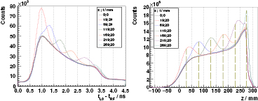
Figure 10. Left: experimental PGT spectra of the L0 detector at  ,
,  cm, for 230 MeV protons and a bone insert inside the full (400 mm) PMMA target at
  (position; thickness as described in figure 1). Spectra are normalized according to dead time and charge, whereas phase drift is corrected manually to match all leading edges. Energy threshold is 1 MeV. Right: time to distance axis conversion from the left PGT spectra after application of stopping power, sensitivity and gamma time of flight corrections, as well as background subtraction. z refers to the depth with respect to the target's front face (beam entrance point). Vertical dashed lines mark the centroid of the bump according to the simBox model.
Download figure:
Standard image High-resolution imageFigure 10 (right) shows a tentative conversion of PGT spectra to depth profiles, after corrections for solid angle effects, attenuation, gamma time of flight and transformation of time to space with the stopping power differential equation as in (Golnik et al 2014, equation (5)). In other words, a simple backprojection is applied to recover the depth profile information from the experimental data. Note that we apply an iterative background subtraction algorithm (Ryan et al 1988). However, at this stage, the space origin is elected arbitrarily and we do not apply a deconvolution with the system time response, which explains the absence of a sharp leading edge at  .
.
For all bone insert measurements (the special case at 269 mm aside), the trailing edge is  mm left from the homogeneous phantom, while the expected range difference is
  8 mm. It is worth pointing out that the a priori assumption of the target geometry, stopping power and time to space conversion curve predetermines (biases) the respective position of the falling edge in figure 10 (right).
The centroid of the bone, namely the space point with the largest surplus in counts with respect to the homogeneous case, is depicted in figure 11 for all locations z of the 20 mm insert. The values expected by the simBox model are in considerable agreement with the experimental ones.
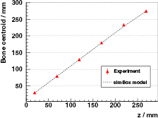
Figure 11. Measured spatial position (centroid of the surplus) of a 20 mm bone insert at different distances z from the PMMA target's front face with the L0 detector, corresponding to the converted spectra of figure 10 (right). The experiment is compared to the values expected according to the simBox model.
Download figure:
Standard image High-resolution image4.5.2. 100 MeV proton energy
Stacked target. For the stacked target experiment at the WPE accelerator (figure 12), analogous to that at the AGOR facility (Golnik et al 2014), one can identify a shift to the right in the peak centroid correlated to the target thickness, as well as an increase in the prompt gamma production (area under the curve). Compared to figure 7, the PGT profile is highly blurred due to the much larger bunch time spread at 100 MeV (see table 3). Nonetheless, we can rely on the analysis of distribution momenta, which retain essential information about the proton range.
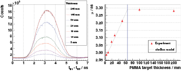
Figure 12. Left: PGT spectra of the B1 detector at  ,
,  cm for 100 MeV protons and different PMMA target thicknesses (listed in the legend). Spectra are normalized according to dead time and charge. Energy threshold is 1 MeV. Right: mean value
  (center of gravity after numerical background subtraction) of the PGT distributions over the target thickness. The experimental data are compared to the values predicted by the simBox model. The blue vertical line marks the range of 100 MeV protons in a full target.
Download figure:
Standard image High-resolution imageFigure 12 (right) evinces the linear relationship between centroid and target thickness until a saturation or plateau is reached, i.e. when the protons are already completely stopped (proton range is 6.5 cm). As in Golnik et al (2014), a reasonable agreement between modelling and experiments is found: when fitting the slope of the left part of the graph, we obtain  ps mm
ps mm for the experiment versus
  ps mm
ps mm for the simBox model. Note that the election of the global time offset in the experiment relative to the model is arbitrary. We select the value maximizing the agreement with all the experimental points.
Air cavities. The influence of tissue heterogeneities is illustrated in figure 13 (left): air cavities of different thicknesses are inserted at a fixed position inside the full PMMA target. On the one hand, the spectrum maximum decreases with increasing thickness of the cavity. On the other hand, the falling edge of the spectrum shifts slightly to the right as a consequence of the overshoot. Thus, at least 5 mm range differences can be distinguished at 100 MeV. The shift to the right in the centroid of the distribution for the 5 mm cavity is  ps for the experiment and
  ps for the simBox model, while for the 10 mm cavity, the experimental shift with respect to the homogeneous case is
  ps versus
  ps for the model.
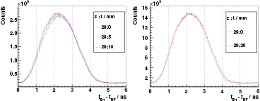
Figure 13. Left: PGT spectra of the B1 detector at  ,
,  cm, for 100 MeV protons and different air cavities inside the full (200 mm) PMMA target at
  (position: thickness as described in figure 1). Spectra are normalized according to dead time and charge. Energy threshold is 1 MeV. Right: equivalent settings, but a single bone insert instead of an air cavity. Spectra are normalized according to their respective maximum.
Download figure:
Standard image High-resolution imageBone inserts. Figure 13 (right) compares a full target PGT spectrum to the case with a 20 mm bone insert at 29 mm depth. The distributions are normalized to their respective maximum, as the higher amount of gammas produced in the heterogeneous case shadows the comparison of the trailing edge of both spectra. We can conclude that a bone insert increases the gamma production rate as well as decreases the width of the time distribution due to the undershoot effect ( 8.5 mm range difference according to stopping power data), which results in an earlier average detection time of the prompt gammas. The shift to the left in the distribution's centroid with respect to the homogeneous case is
  ps for the experiment and
  ps for the simBox model.
5. Discussion
Motivation. A main purpose of the present experiment is the estimation of the minimum range difference that generates a measurable change in the shape of the PGT spectrum, rather than the quantitative retrieval of the range. The setup is optimized for timing but is not intended for high rate measurements or long-term detector gain stability. This is considered as a further step once the suitability of PGT in clinical environments is shown at all.
Systematic program. Proton range variations due to a stacked PMMA target as well as cavity and bone heterogeneities are detected. In most cases, an energy threshold of 1 MeV is applied to the data for maximizing the statistics, despite the fact that the correlation of the gamma emission profile with the dose is higher for an energy threshold of 3 MeV (Verburg et al 2013). For 100 MeV proton energy, range differences of 5 mm can be successfully retrieved (without any sophisticated numerical analysis). These are identified qualitatively based on the distinctness of the spectra compared to the homogeneous case. The quantitative assessment relies on the comparison of distribution momenta between experiment and simBox model, with overall reasonable agreement. There are some systematic deviations in certain cases, either due to bunch-to-RF phase drift or because of the oversimplified model.
For an energy of 230 MeV, the much lower bunch time spread allows to recover information across the shape of the PGT spectra and not just through distribution momenta. This could be deployed for depth-emission profile reconstruction with a single detector, a milestone in the field of in vivo proton dose verification. Figures 9 and 11 demonstrate the potential for differentially correlating time to depth, and imply a qualitative leap forward of the PGT method with respect to Golnik et al (2014), notwithstanding the need of more advanced conversion tools.
First tested at the AGOR research accelerator, the robustness of the PGT method is examined in terms of background, bunch time spread and bunch stability during the experiments in clinical facilities. In this scenario, we encounter several factors limiting the accuracy of PGT in its simplest form. First attempts to understand and quantify these effects are described, and strategies to circumvent them are proposed.
Bunch structure. The bunch spread is measured indirectly with a thin PMMA target. Together with the prompt gammas, there is a high background of scattered protons. This motivates the use of dedicated charged particle detectors in upcoming experiments to determine the bunch width (and phase) directly from protons, e.g. those scattered in the beam exit window.
The increase of the bunch time spread at lower energies is an intrinsic hurdle for the PGT method at the widespread C230 (and, in general, at other clinical fixed-energy cyclotrons relying on a degrader to brake the ions), compared to the AGOR research accelerator. As a consequence, PGT spectra revealing valuable profile information at 230 MeV due to a low bunch time spread may blur completely at 160 or 100 MeV, which are proton energies much more frequent in an actual therapeutic irradiation. Strategies like the reduction of the momentum slit opening suggest that there is still room for improving the system time resolution, or even for optimizing the time spread in future designs of clinical isochronous cyclotrons.
Some research cyclotrons (like AGOR) do not require an energy selection system, as they vary magnetic field and radio frequency to provide just the desired beam energy, but are not usual in the clinics. Rather, fixed-energy isochronous cyclotrons are a widespread choice in hospitals. Synchrotrons or synchrocyclotrons are also available (or planned) in a few treatment centers. A priori, the application of the PGT method at these synchronous accelerators, where the micro bunch time spread may be large and the instantaneous current higher, is not straightforward and has to be explored.
Phase drift. The main burden that affects the experimental data presented in this paper is the bunch phase drift with respect to the RF signal, which prevents us from making further quantitative analysis on centroid shifts. To overcome this instability experimentally, we are currently developing a bunch phase monitor based on phoswich detectors (Wilkinson 1952), which could identify and select by energy the protons scattered at the beam exit window, and measure their crossing time. Then, the actual shift between bunch and RF can be subtracted from the PGT spectra. Additionally, the measurement of the temporal shape of the beam bunch (non-Gaussian shape) is essential for the modelling, in order to apply a convolution with the proper system response.
Within a clinical pencil beam scanning session (few seconds), the effect of long-term bunch drift is expected to be negligible when comparing consecutive spots. Rather, one has to correct the mean drift (and variation of bunch time spread) when comparing the experimental results of two different treatment fractions (one day separation). Moreover, for the comparison of PGT spectra with modelled ones, one has to discriminate the different energy layers within the fraction, as the crossing time of the beam exit window with respect to the RF signal depends on the beam energy (and beam line length). This has to be calibrated accurately beforehand, or monitored with the aforementioned phoswich detector for each energy layer in real-time.
Normalization. The uncertainty of the normalization factor to number of protons is also a major hurdle to the presented data, but is a circumstantial limitation of the dead time model. We expect this provisional problem to be solved with upgraded electronics.
Background. Significant background radiation due to scattered charged particles, neutrons and material activation is observed in the experiments, specially for high proton energies. The PGT method has proven robust for retrieving range shifts in most cases, but the pedestal present in the time histograms is still an important concern. A low signal to noise ratio is observed for the thin target measurements. For thicker targets, the background has a particular (not flat) time structure. Efforts have to be undertaken to either reduce physically the background, or to model and subtract it for minimizing the bias on the retrieved range shift.
Detector geometry. For detectors placed downstream, suppression of charged particles, e.g. by pulse shape discrimination, is advisable to reduce the high relative background generated by scattered protons (as observed in the energy over time spectra). Nevertheless, an upstream positioning provides in principle a better performance, as the gamma time of flight to the detector extends the PGT spectrum and thus allows to resolve more details. In addition, the inherent fast neutron background is lower in backward direction (Gunzert-Marx et al 2004). The drawback is that a high percentage of the measured gammas stem from the target's front face rather than from the Bragg peak position due to a different solid angle coverage. In cases where the accumulated statistics is low, this may be a limitation if a reconstruction of the particle range based on the trailing edge of the PGT spectra is attempted.
Throughput. The measurements described in this paper are made with a pencil beam current between 10 and 100 pA and a duration of 5 to 7 min. Let us give some numbers for a concrete case: the irradiation of a full PMMA target at 160 MeV proton energy. The acquisition lasts 6.5 min and the delivered charge is 23 nC, corresponding to  protons and a beam current of 59 pA. Assuming an isotropic prompt gamma yield of 0.16 as in Golnik et al (2014), the emission rate of prompt gammas with energies higher than 1 MeV is
  s
s . The solid angle covered by the L0 detector at 30 cm distance from the ring center is
  , the minimum detection efficiency is
  (Berger et al 2010) and the gamma attenuation inside the target is of the order of 45% (Hubbell and Seltzer 2004). The resulting overall efficiency
  is
is  and the measured detector trigger rate is 33 kcps. In our particular acquisition system, as the dynamic dead time is 34%, the acquisition rate is 22 kcps and the total number of registered events is
  . Thus, the dynamic efficiency is
  . Note that we dismiss background contributions for this calculation.
Besides the bunch time spread, detector throughput is the critical parameter for PGT and has to be addressed for obtaining a reliable range measurement in real-time and in vivo. The electronics required to cope with high count rates up to 1 Mcps without detector overload are under development.
Statistics. What would be the differences in a clinical treatment plan compared to this experiment? Concerning a realistic 2 Gy irradiation fraction with  protons (in total) delivered to a small area of the brain with pencil beam scanning at an IBA C230 machine, the instantaneous current at nozzle exit during spot delivery is around 2 nA, i.e.
  p s
p s (Perali et al 2014). A typical pencil beam spot is thus delivered within a few milliseconds. Note that the overall treatment fraction duration includes the times necessary for magnet sweeping between the spots and for energy switching between the layers, that are dependent on the actual treatment plan. Therefore, we base our rate estimates on proton beams of 2 nA peak current measured at nozzle exit.
If we consider the L0 detector setup described above ( ) without dead time effects, the resulting acquisition rate is
  1 Mcps (no overload expected with upgraded electronics), i.e 500 kcps nA
 . The planned number of protons per spot is
  for
for  75% of the spots. In other words,
  2000 gammas are measured for each raster point, so that the analysis of the PGT spectrum seems not realistic on a single spot basis due to insufficient statistics. Rather, one should collect data from several detectors or accumulate gamma rays from neighbour spots in a single spectrum.
How do we quantify this qualitative statement? The statistics necessary for detecting a range shift with 2 mm precision in a PGT spectrum depending on beam current and proton range has been analysed in Golnik et al (2014) based on the theoretical error of distribution momenta. Equivalent conclusions could apply here for 100 and 160 MeV proton energies. In the case of low bunch spread (230 MeV protons), one may want to retrieve a range difference based on the shift of the falling edge (see figure 8), which corresponds to the Bragg peak region, instead of on the mean value or distribution's width. What is the minimum number of gammas in the PGT spectrum for detecting a range shift in this case? There is no general answer for this question, as the detector orientation, target attenuation and amount of background may play a significant role on the shape of the falling edge.
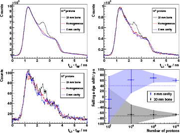
Alternatively, we perform a statistical analysis on experimental data of the L0 detector for 230 MeV protons and three particular target configurations: (a) a full homogeneous PMMA phantom, (b) a 5 mm air cavity inside it, and (c) a 20 mm bone insert in place of the cavity.
The original histograms (complete measurements) have around  entries each. Once the region of interest (the fall-off) inside the three PGT spectra is defined, the trailing edge deviation is calculated by finding the virtual time shift on (a) that minimizes the weighted χ2 test between the (a)–(b) histograms for the cavity or (a)–(c) for the bone insert. These χ2 tests are performed for four different statistical sample sizes (random subsets of the whole measurement):
  ,
,  ,
,  and
and  histogram entries (prompt gammas plus background). Assuming for simplicity the aforementioned efficiency
  , these virtual measurements would correspond approximately to an irradiation with
  ,
,  ,
,  and
and  protons, respectively. For each case, 100 subsets of equal sample size are selected randomly in order to determine the average time shift and the standard deviation.
Figure 14 shows the complete statistical study. One can see how the reduction of sample size (number of protons) degrades the shape of the PGT spectra. Statistical noise hampers the identification by eye of the shift of the falling edge the lower the number of protons. On the basis of the χ2 numerical analysis (bottom right plot of figure 14),  protons seem to be the threshold for determining a 5 mm shift of the falling edge in a single spot. Below this boundary, namely the region enclosing most of the clinical spots, the statistical deviation is too high, as illustrated by the overlapping of the coloured uncertainty areas. Looking at the error bars, a range shift down to 2 mm can be identified with
  protons. It is worth to remember that these considerations apply for a particularly low bunch spread scenario (230 MeV), a single detector in upstream orientation and selected target configurations.
Figure 14. Top row and bottom left plot: PGT spectra of the L0 detector at  ,
,  cm, for 230 MeV protons. The homogeneous case (red curve) corresponds to a full PMMA target (400 mm). A heterogeneous slice is placed inside the full PMMA target at
  mm;
mm;  mm (air cavity—blue curve) or
  mm;
mm;  mm (bone insert—black curve), where
  are the (position: thickness) as described in figure 1. Energy threshold is 1 MeV. Spectra of top left figure are normalized to their respective maximum and shifted in time to match their leading edges at 50% of the rise. The obtained shift and scale factors are applied then for the top right and bottom left plots. A smoothing filter is applied on the histogram bin contents for visual enhancement (not used later in numerical analysis). The legend header contains the number of protons associated to each spectrum (assuming
  ). Bottom right: shift of the falling edge (retrieved with the weighted χ2 test) with respect to the homogeneous case depending on the number of protons. Experimental points are averaged over 100 samples of equal size (see text), being the vertical error bars and enclosing solid area the standard deviation. The horizontal error bars are set to 30% of the number of protons. The dashed lines depict the expected shift of the trailing edge according to the simBox model:
  ps for a 5 mm overshoot due to the cavity and
  ps for a
  8 mm undershoot due to the bone insert.
Download figure:
Standard image High-resolution image
How could we increase the collected statistics? One may enlarge the detector volume at the price of developing electronics that sustain a higher throughput. One could also sum up data from several detectors or from neighbour spots to recover statistics, or consider a downstream detector, that maximizes the solid angle at the Bragg peak. More sophisticated numerical analysis including the whole histogram for the shift retrieval instead of just a region of interest is also advisable. For example, in our χ2 tests, we waste useful information like the difference in the gamma production at the location of the heterogeneity, which is still visible in the bottom left plot of figure 14. There is undoubtedly room for improvement.
An opposite approach, which would affect clinical workflow and planning, is to deliver a benchmark spot at the distal region, namely the raster point of the plan with the highest number of protons. The rationale is to detect with confidence (along the selected incidence direction) potential range shifts due to anatomy changes between treatment fractions. The number of protons of the richest spot depends on each particular tumour location and treatment planning software, but it is not uncommon to have at least one spot with  protons, see (Smeets et al 2012), figure 19. One could deliver this benchmark spot immediately at the beginning of the treatment and check the acquired PGT spectrum. If no deviations are observed, one would consecutively repeat this step for all spots of the distal layer to cover other irradiation areas. If the results comply with the expectations, one could then deliver all remaining spots of the plan. Hence, just the spot order delivery but not the dosimetry is affected.
Another option would be to double the detector size and halve the instantaneous clinical current (for all spots) to keep the count rate at an acceptable level, but multiply the detection efficiency  by a factor of two. For the particular treatment plan considered above (
 protons at
  p s
p s ), the actual irradiation time of the small area of the brain lasts about one second. This irradiation time is relatively small compared to the global delivery time (
 15 s), with a significant dead time due to magnet sweeping and change of energy layers. Hence, halving the beam current would not increase significantly the treatment duration in the WPE treatment facility.
A further strategy, which combines the two last, is to deliver at treatment beginning the spot with the highest number of protons of the plan, e.g.  protons, with a very low beam current (one proton per bunch, around 1 s irradiation at 2 pA) and measure the passage of every proton with a beam hodoscope. The added value is that the effect of bunch time spread is suppressed for any beam energy, as each detected prompt gamma can be correlated to the primary proton. The collected statistics can also be maximized as the lower beam current allows the use of larger detectors.
Quantification. For the quantitative retrieval of the range, either directly or by comparing with the expected PGT profile, an extensive simulation and modelling based on section 3.7 is under progress. More realistic PGT modelling should consider effects like energy-resolved emission profiles, detector sensitivity for complex geometries, background subtraction and non-Gaussian temporal system response.
Stopping power. The PGT spectra at 230 MeV (low bunch spread scenario) do not provide a proportional image of the gamma emission but rather a stretched one. An inverse transformation is needed as intermediate step if one wants to obtain a depth profile, see figure 10. However, this calibration depends on the accurate knowledge of the stopping power of the traversed tissue (Golnik et al 2014). One may then argue that no method for detecting range uncertainties should depend on their most common source: the variation of the tissue composition (stopping power) between clinical fractions. The absence of a daily patient imaging prevents a recalibration of the time to space relationship for each fraction. Does this mean that the PGT approach is useless?
Let us put it the other way round and calculate a PGT spectrum according to the treatment plan expectations (and uncertainties). If, unluckily, the assumed anatomy is inaccurate, the reference PGT profile will be biased. As a consequence, an overshoot of e.g. 5 mm may occur and the measured PGT profile will change with respect to the expected one due to its dependence on the spatial emission profile, but also on the stopping power itself (simultaneous dependency). Due to the unawareness on the exact anatomy and the bias introduced on the reference spectrum, one may not be able to quantify with utmost accuracy the actual range deviation. But we believe that the differences (in shape or momenta) between the reference and the measured spectra could be blamed (with enough confidence) on e.g. a shift between 3 mm up to 7 mm. In other words, the PGT method could serve as real-time safety assurance for detecting severe deviations rather than accurate range measurements. This strategy is also applicable for lower proton energies (larger bunch spread).
In any case, even for an ideal prompt gamma camera that reproduces the spatial emission profile faithfully (without distortions) and with perfect counting statistics, the amplitude of the actual range shift is biased by the treatment plan expectations. The reason is that the correlation of prompt gamma yield to particle range depends on the assumed tissue composition. Still, experimental measurements that reveal significant differences with respect to biased reference spectra are a reliable indicator that something is not going as planned.
Outlook towards the clinics. At this stage, the experimental results do not allow a comparison of the PGT method with other more developed techniques as e.g. the knife-edge slit camera, which is able to image millimetre shifts at clinical current intensities (Perali et al 2014). Our method is far beneath in the ladder of clinical translation, and one can think of many limiting scenarios in which its applicability is questionable or yet unproven. However, some trends and qualitative aspects are already observed in this work, which encourage the hope of a quantitative retrieval of the range based on the PGT method. Whereas we can not claim a spatial precision comparable to other methods on a single spot basis, we believe that the much lower expense and footprint of this technology may boost the applicability and spread of this technique in the clinics, and thus deserves further investigations.
Thanks to its real-time range assessment capability, we consider that PGT has the potential to be translated into clinical practice as a fast handle to stop a running treatment with significant deviations during the clinical fraction. The workflow for detecting severe range shifts could look like:
- A realistic spatial emission profile is simulated according to the treatment plan.
- The expected timing profile is calculated based on the detector model and patient data.
- PGT spectra are measured during the clinical fraction and corrected for bunch drifts (with respect to the previous treatment session) by a phase monitor.
- The center of gravity of the modelled and measured PGT spectra is compared in real-time.
- If the difference exceeds a clinically critical value, the treatment can be interrupted and the source of error analysed or corrected in the upcoming treatment fractions.
6. Conclusions
In vivo range verification in real-time is a must for improving the outcome of ion beam therapy. The prompt gamma rays produced in nuclear interactions are reliable signatures for reconstructing the depth-dose profile, provided that the tissue composition is well known. The prompt gamma ray timing method aims at assessing the range based on a simple detector setup without mechanical collimation.
This paper describes the first tests of PGT at a clinical proton accelerator with different phantoms and detectors. The bunch time spread is characterized for different energies and the robustness of the method concerning background and bunch stability is investigated. For  protons (230 MeV energy) and a single detector, particle range differences of 2 mm are identified in predefined heterogeneous targets based on the distinctness of timing distributions. For
  irradiated protons, a 5 mm range shift is retrievable by numerical analysis. The experimental results also prove that PGT spectra comprise very detailed information on gamma emission along the track when the bunch spread is low.
The PGT method appears to be feasible in a clinical scenario with a pencil beam if following intermediate steps concerning hardware, software and procedure are addressed to counteract the encountered limitations:
- Addition of a bunch phase monitor which measures the long-term drift with respect to the accelerator RF as well as the bunch temporal shape for each treatment fraction. The monitor can also correlate the crossing time of the protons through the beam exit window with respect to the RF for each energy layer.
- A much higher detector and data acquisition throughput to cope with the gamma rate expected in an actual clinical treatment fraction.
- An accurate time spectrum and background modelling, and numerical analysis or even iterative algorithms for obtaining a quantitative measurement of the particle range.
Experiments with improved detectors and electronics, realistic currents, beam scanning and anthropomorphic phantoms are the next steps towards clinical translation.
In conclusion, the overall experimental results underline the potential of the prompt gamma ray timing method for range assessment in a clinical pencil beam and reassure this novel approach as a promising alternative in the field of in vivo dosimetry.
Acknowledgments
This work is supported by the German Federal Ministry of Education and Research (BMBF-03Z1NN12) and by the European Commission within the Seventh Framework Program through ENTERVISION (grant agreement number 264552). We thank M Berthel, A Dreyer, A Hartmann, K Heidel, A Junghans, M Kempe, T Kormoll, A Laso-García, M Sobiella and D Weinberger for the excellent assistance, and the staff of the ELBE and WPE facilities for their support.