


Abstract
This survey is devoted to results related to metric properties of classical continued fractions and Voronoi–Minkowski three-dimensional continued fractions. The main focus is on applications of analytic methods based on estimates of Kloosterman sums. An apparatus is developed for solving problems about three-dimensional lattices. The approach is based on reduction to the preceding dimension, an idea used earlier by Linnik and Skubenko in the study of integer solutions of the determinant equation  , where
  is a
is a  matrix with independent coefficients and
  is an increasing parameter. The proposed method is used for studying statistical properties of Voronoi–Minkowski three-dimensional continued fractions in lattices with a fixed determinant. In particular, an asymptotic formula with polynomial lowering in the remainder term is proved for the average number of Minkowski bases. This result can be regarded as a three-dimensional analogue of Porter's theorem on the average length of finite continued fractions.
Bibliography: 127 titles.
Export citation and abstract BibTeX RIS
§ 1. Introduction
1.1. Linnik's problem
Many number-theoretic problems can be reduced to the study of a Diophantine equation

where  is a homogeneous polynomial and is an integer. The only general method that makes it possible to describe the asymptotic properties of solutions of equation (1.1) is the Hardy–Littlewood circle method, which, however, requires additional properties of the polynomial (see [1]). In certain situations the distribution of the solutions of (1.1) can be investigated by methods of algebraic number theory and algebraic geometry (see [2], [3]), but in the general case one does not even know estimates of the correct order for the number of solutions.
If equation (1.1) defines a homogeneous variety with an action of a linear algebraic group, then the possibility arises of applying methods of harmonic analysis on this group (see [4]–[7]). An important special case of such a situation is the determinant equation

where is a square matrix with independent coefficients. For matrices Linnik and Skubenko [8] (see also [9], Chap. VIII) proved that as  the integer solutions of equation (1.2) are uniformly distributed with respect to the Haar measure. They were solving the problem under the assumption that the normalized matrix
  is contained in some fixed domain
  of finite measure. They proved an asymptotic formula for the number of solutions of (1.2) without explicitly indicating a lowering in the remainder term. (An explicit estimate for the remainder term for the domain
  , where
  is the Euclidean norm, was given in [10].) In the general case the problem of the distribution of the integer solutions of equation (1.1) is known as Linnik's problem and is also usually considered under the assumption that
  , where
  is the degree of the polynomial (see [4], [5], [10]). See [11]–[14] for development of the method of Linnik and Skubenko.
1.2. Linnik–Skubenko reduction
By Weyl's criterion (see, for example, [15]) a necessary and sufficient condition for the uniform distribution of a system of functions  is that
where  are arbitrary integers that are not simultaneously equal to zero, and
  . This condition makes it possible to reduce the study of the uniform distribution of systems of functions to estimates of the corresponding trigonometric sums.
Many problems related to planar integer lattices (see details in §2.2) can be reduced to the investigation of solutions of the determinant equation
This equation can be replaced by the equivalent congruence

assuming that  is fixed and that the value of
  is determined from the equation
  .
.
By using Weyl's criterion the problem of the uniform distribution of solutions of the congruence (1.4) can be reduced to estimates of the sums
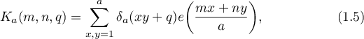
where  are arbitrary integers,
  is a positive integer, and
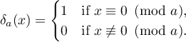
  is the characteristic function of divisibility by :
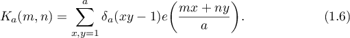
For  the sums (1.5) coincide with the classical Kloosterman sums
Non-trivial estimates are known for the sums (1.6) and (1.5), and this makes it possible to find asymptotic formulae for sums of the form

by replacing them with the corresponding integrals. Problems in the geometry of numbers, the theory of continued fractions, and so on, can be reduced to the calculation of similar sums (see the survey [16]).
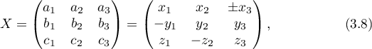
In the three-dimensional case, bases of lattices with determinant are parametrized by solutions of the determinant equation (1.2), where is a matrix of the form
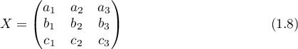
in which the coordinates of the basis vectors are written in columns. In the study of Voronoi–Minkowski three-dimensional continued fractions (see the original publications [17], [18], and [19], as well as their exposition in [20], [21], and [22]), the necessity arises of counting the solutions of (1.2) for which the normalized matrix can vary in a domain of infinite measure.
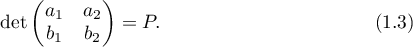
The Linnik–Skubenko method was based on reduction to the preceding dimension — to the determinant equation (1.3). The main idea was that if the matrix  is fixed and has non-zero determinant
  , and
, and  , then for each solution (1.8) of equation (1.2) it is possible to construct a series of solutions
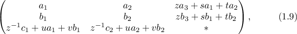
where  ,
,  , and
, and  are arbitrary integers. The presence of the parameter
  , which is non-linearly involved in the parametrization (1.9), makes it possible to use Kloosterman sums for reducing the problem of the distribution of the solutions of (1.2) to sums of the form (1.7), the methods of calculation of which are well known.
In [23] a more precise version of the Linnik–Skubenko reduction was proposed which is applicable, in particular, for domains  of infinite volume. The auxiliary two-dimensional problems arising after the reduction were solved in [24]. In the present paper the results in [23] and [24] are applied to the study of statistical properties of Voronoi–Minkowski three-dimensional continued fractions. One can expect that the proposed approach will turn out to be useful also for solution of other problems related to three-dimensional lattices.
1.3. Theorems of Heilbronn and Porter
For a rational  , let
, let  denote the length of the expansion of into a finite continued fraction
where  (the integer part of ),
  are positive integers, and
  for
for  .
.
Heilbronn [25] proved an asymptotic formula for the average value of taken over rational numbers with a fixed denominator:
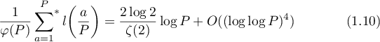
(henceforth an asterisk means that the summation is carried out over the reduced system of residues). Porter later [26] refined this result by isolating the next significant term, which is an absolute constant:
(we denote by  a polynomial of degree
  in a variable
  ; the constants in the symbols
  are always assumed to depend on an arbitrarily small positive number
  ). Heilbronn's proof is elementary. Porter used estimates for Kloosterman sums and estimates for trigonometric sums according to van der Corput.
1.4. Brief statement of the main result
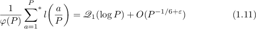
In the present paper the refined version in [23] of Linnik–Skubenko reduction is used to construct a method of analysis of minimal bases in three-dimensional lattices. In particular, this method enables us to prove a three-dimensional analogue of Porter's result (1.11) for them.
Theorem 1.1. The average number of Minkowski bases over totally primitive lattices with determinant has the asymptotics

A more precise statement of this result will be given below after the definitions of all the requisite notions (see Theorem 3.3 below). From the viewpoint of Linnik's problem, the presence in the asymptotics of a polynomial of second degree in the logarithm of is explained by the fact that when counting solutions of the equation one has to deal with a domain of infinite volume on the variety defined by the equation  .
.
A three-dimensional analogue of Heilbronn's theorem (1.10) was proved by Illarionov [27] (see [28]–[30] concerning other multidimensional generalizations). Illarionov's arguments make it possible to determine the leading term in the asymptotic formula (1.12) with remainder  .
.
Equation (1.11) can be interpreted as a formula for the average length of the Euclidean algorithm applied to a pair of numbers  such that
  and
and  . From the geometric viewpoint, the left-hand side of equation (1.11) can be understood as the average number of minimal bases in lattices with bases from the pair of vectors
  and
and  . The formula (1.12) describes the average number of minimal bases in three-dimensional lattices generated by the vectors
  ,
,  , and
, and  (see §2.3). The same quantity can be interpreted as the average number of all possible bases that can appear in the Euclidean algorithm applied to a triple
  in which
  and
and  .
.
1.5. Plan of the paper
In §2 we give a brief survey of results connected with the metric theory of infinite and finite continued fractions.
In §3 we discuss three-dimensional continued fractions according to Voronoi and Minkowski. The precise statement of the main result is given.
In order to illustrate the scheme of the proof of the main theorem, we briefly describe in §4 the main steps needed to solve a model problem — the proof of a simplified version of equation (1.11). The general scheme of arguments in the proof of the main Theorem 3.3 is the same.
In §5 the solutions of equation (1.2) are divided into groups, in each of which the solutions will be counted independently (until a certain moment). At the end of §5.3 we describe the detailed scheme of proof of the main result.
In §§6–8 asymptotic formulae are proved for the number of solutions of equation (1.2) with fixed corner element  and with corner minor
  , by three different methods.
§ 2. Metric properties of continued fractions
2.1. Gauss measure
The metric theory of continued fractions goes back to Gauss' problem on the typical behaviour of numbers of the form

where ![$\alpha=[0;a_{1},a_{2},\dots]$](https://content.cld.iop.org/journals/0036-0279/70/3/483/revision1/RMS_70_3_483ieqn57.gif) is a random number in the interval
is a random number in the interval  and
and  is the Gauss map:
For a real number ![$\xi\in[0,1]$](https://content.cld.iop.org/journals/0036-0279/70/3/483/revision1/RMS_70_3_483ieqn60.gif) , let
, let  denote the measure of the set of numbers
  for which
  . In studying iterations of the map , Gauss arrived at the conjecture that

(this is known from the correspondence of Gauss with Laplace; see [31], Chap. 3). Kuz'min [32] obtained the asymptotic formula

from which Gauss' conjecture follows. Kuz'min's result was refined by Lévy [33] and Wirsing [34]. The definitive solution of Gauss' problem is due to Babenko [35]. He proved the existence of an infinite sequence of numbers  decreasing to zero,

and a corresponding sequence of analytic functions  such that
Equation (2.1) means that the typical behaviour of the numbers  is described by the Gauss measure
which is invariant under the map . In particular, this implies that the probabilities of the appearance of positive integers  as partial quotients of real numbers are described by the Gauss–Kuz'min distribution

In many cases it is more convenient to consider the extended Gauss measure

which is invariant under the map
(see [36]), which is almost everywhere invertible. If we expand the coordinates of the initial point  into continued fractions

then on the doubly infinite sequence  obtained by concatenation of the expansions (2.5) written in opposite directions the map
  is equivalent to a shift:
  , where
  is an arbitrary integer,
 ![$\alpha_n=[0;a_n,a_{n+1},\dots]$](https://content.cld.iop.org/journals/0036-0279/70/3/483/revision1/RMS_70_3_483ieqn73.gif) , and
, and ![$\beta_n=[0;a_{n-1},a_{n-2},\dots]$](https://content.cld.iop.org/journals/0036-0279/70/3/483/revision1/RMS_70_3_483ieqn74.gif) .
.
2.2. Statistical properties of finite continued fractions
A discrete version of Gauss' problem is to study the statistical properties of finite continued fractions. For rational numbers (as well as for real numbers) it is convenient to interpret the Gauss–Kuz'min statistics in a wider sense. For real ![$\xi,\eta\in[0,1]$](https://content.cld.iop.org/journals/0036-0279/70/3/483/revision1/RMS_70_3_483ieqn75.gif) and rational , we define the Gauss–Kuz'min statistics by the equation
and rational , we define the Gauss–Kuz'min statistics by the equation
We assume that an empty continued fraction is equal to zero by definition. If  is some condition, then
 ![$[A]$](https://content.cld.iop.org/journals/0036-0279/70/3/483/revision1/RMS_70_3_483ieqn77.gif) is the characteristic function of the set defined by this condition:
is the characteristic function of the set defined by this condition: ![$[A]=1$](https://content.cld.iop.org/journals/0036-0279/70/3/483/revision1/RMS_70_3_483ieqn78.gif) if the condition holds, and
if the condition holds, and ![$[A]=0$](https://content.cld.iop.org/journals/0036-0279/70/3/483/revision1/RMS_70_3_483ieqn79.gif) otherwise. In particular,
otherwise. In particular,  .
.
The distribution of the partial quotients in the expansion of numbers  in the case where
  and was first studied in 1961 by Lochs (see [37], as well as [25], [38]). Later this problem was posed in a more general setting by Arnold as Problem 1993-11 in [39] (the papers [40]–[45] were devoted to Arnold's problem). Lochs' result can be interpreted as follows: the asymptotic formula
holds for the average value of the Gauss–Kuz'min statistics (2.6) in which the leading coefficient is proportional to the Gauss measure of the rectangle ![$[0,\xi]\times [0,\eta]$](https://content.cld.iop.org/journals/0036-0279/70/3/483/revision1/RMS_70_3_483ieqn83.gif) .
.
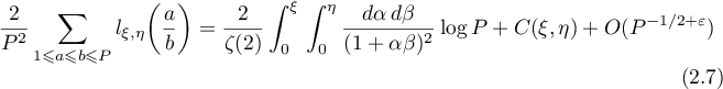
The function  , as well as the left-hand side of equation (2.7), is discontinuous at all the points that have at least one rational coordinate. This function is defined by a singular series, that is, a series consisting of the remainder terms of asymptotic formulae (see [37], [44], [46], [47]).
Equation (1.11) can also be generalized to the case of the Gauss–Kuz'min statistics:

(for  the proof is given in [43]; the formula for the principal term follows from Heilbronn's result [25]; the functions and
  can be expressed in terms of each other). By comparing (2.2) with (2.7) (or with (2.8)) we can conclude that the principal terms in the continuous and discrete problems are proportional and are determined by an invariant measure, while the next significant terms differ and are of a fundamentally different nature.
The analytic apparatus used in the study of statistical properties of finite continued fractions makes it possible to solve also other problems in which continued fractions are used as an auxiliary tool.
In particular, this makes it possible
 to analyse the typical behaviour of the Euclidean algorithms with rounding off to the nearest integer [48], [49], with even and odd partial quotients [50]–[52], with by-excess division [53], [54], and with subtractive division [55], [56], and to analyse the typical behaviour of Minkowski diagonal fractions [57] and continued fractions of more general form [58], as well as to study continued fraction expansions of quadratic irrationals [45];
to find the distribution density in Sinai billiards (circular scatterers are placed at nodes of the lattice  ) of the random variable equal to the length of the free path of a particle [59]–[62], and (in an equivalent problem) to calculate the joint distribution density of the lengths of neighbouring segments connecting the origin with primitive points of the integer lattice [63], [64];
to describe the limit distribution of Frobenius numbers with three arguments [65]–[69];
to prove the existence of a limit distribution density for partial Gauss sums and partial theta-series [70]–[72], and also to find these densities [73].
It should be pointed out that for all the problems listed above there exist other approaches based on ergodic theory and methods of the geometry of numbers. Ergodic methods usually turn out to be applicable in a more general situation, but in comparison with analytic methods they require averaging over a greater number of parameters and produce less accurate remainder terms.
In particular, by using ergodic theory it is possible
to analyse a wide class of Euclidean algorithms [74]–[76];
to study Sinai billiards in spaces of arbitrary dimension [77], [78], and to study the behaviour of the free path of particles in quasi-crystallic structures [79];
to prove the existence of a limit distribution density for Frobenius numbers with an arbitrary number of arguments [80], and to describe the properties of this density [81]–[83];
to obtain results on the behaviour of partial Gauss sums and partial theta-series [84], [85].
2.3. Totally primitive lattices
Let  denote the matrix in which the coordinates of the vectors
  are written in the columns. A full lattice
  with basis
  is said to be totally primitive if for every row of the matrix the minors corresponding to the elements of this row are setwise coprime. For example, for a matrix this condition means that
 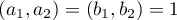 , that is, for
  the notions of primitive and totally primitive lattice coincide. If
  , then for a basis matrix of the form (1.8) the condition of being totally primitive is written in the form
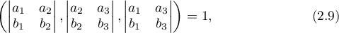
An equivalent definition of a totally primitive lattice is obtained if the lattice is required to have a basis with a matrix
where  and . In particular, this implies that there exist
  three-dimensional totally primitive lattices with determinant .
From the viewpoint of the theory of Diophantine approximations, the local minima of a lattice with basis matrix (2.12) are the best approximations of the linear form  . All that was said above about primitive three-dimensional lattices can be extended in obvious fashion to the case of arbitrary dimension
  .
.
2.4. Multidimensional analogues of the Gauss measure
The Gauss measure is a special case of a more general construction. The set of bases in  -dimensional lattices can be identified with the set of matrices
  . The definitions of local minima and minimal systems of vectors (see §3.1) are independent of the choice of scales on the coordinate axes, and therefore for studying the properties of minimal bases it is natural to consider the quotient space
  , where
  is the group of diagonal invertible
  matrices with real coefficients. The bi-invariant Haar measure on
where  and
and  is the Lebesgue measure, induces on
  the quotient measure
  , which is a right Haar measure and which remains invariant under the left action of :
for any  and
and  .
.
Setting  , where
  for
for  , we can define the measure in the chart
  by
by

Then the right invariance of follows from the formula
in which  is the Haar measure on .
For the measure , taken on the space of matrices of the form  (normalized Voronoi matrices), coincides up to the normalizing factor
  with the extended Gauss measure (2.4). For the measure arises in the study of the statistical properties of Klein polyhedra (see [86], [87]) and Voronoi–Minkowski continued fractions (see [27]). An essential difference between these two objects is the fact that Klein polyhedra are parametrized by the points of the whole space , the measure of which is infinite, while to non-degenerate minimal systems of vectors (that is, systems whose matrices have non-zero determinant; see §3) in the space there corresponds a domain of finite measure : if a matrix with diagonal dominance (in each row the absolute values of the non-diagonal elements do not exceed the absolute value of the diagonal element) defines a non-degenerate minimal system of vectors of a lattice
  , then by Minkowski's convex body theorem,
  and
and
§ 3. Continued fractions and lattices
3.1. Geometry of continued fractions
There are two geometric interpretations of classical continued fractions admitting a natural generalization to the multidimensional case. In the first, due to Klein (see [88], [89], and also an earlier remark of Smith [90], pp. 146–147), a continued fraction is identified with the convex hull (the Klein polygon) of the points of the integer lattice that lie in two adjacent angles. The second interpretation, proposed independently by Voronoi and Minkowski (see [17], [18] and [19], [91], as well as the reiteration of the original results in [20], [21], and [22]), is based on the use of local minima of lattices, minimal systems, and extremal parallelepipeds (see the definitions below). In planar lattices the vertices of Klein polygons (after a linear transformation taking the sides of the angles to coordinate axes) can be identified with Voronoi local minima. But the geometric constructions of Klein and Voronoi–Minkowski become different starting from dimension  (see [92], [93]).
We recall the requisite definitions going back to Voronoi and Minkowski. A lattice  is said to be irreducible (or a lattice of general position) if the coordinate hyperplanes do not contain nodes of the lattice other than the origin; in the opposite case the lattice is said to be reducible. The set of full -dimensional lattices (that is, lattices of dimension coinciding with the dimension of the space) is denoted by
  , and the subset of it consisting of irreducible lattices by
  .
.
For a non-empty finite set  , we put
In other words,  is the smallest parallelepiped circumscribed around the set (we consider only parallelepipeds with centre at the origin and with faces parallel to the coordinate planes).
A system of nodes of order of a lattice (not necessarily a full lattice) is defined to be any finite -tuple  of non-zero nodes of in which
  (
( ). With an arbitrary system
  we associate the matrix
  by writing the coordinates of the vectors
  in the columns.
A node  of a lattice
  is called a Voronoi relative (local) minimum of (henceforth, simply a minimum) if the parallelepiped
  does not contain nodes of other than its own vertices and the origin (see [18]). The set of all local minima of is denoted by
  . If has several minimal vectors
  such that
  (
( ), then we agree to include in
  only one of these vectors.
A system  of vectors of the lattice is said to be minimal if the parallelepiped
  does not contain nodes of other than the origin. In particular, for irreducible lattices the notion of a minimal system of order
  coincides with the notion of a local minimum. For reducible lattices the definition of a minimal system has to be made more precise (see [94]).
In the two-dimensional case we introduce on the set of local minima the structure of a sequence

in which the vectors  (
( ) are ordered by decrease of the first coordinate:
  ,
,  . Here every minimal pair of vectors has the form
  (that is, consists of neighbouring local minima) and is a basis of the lattice (see [18]); such pairs are called Voronoi bases.
By considering the normalized matrices

we deduce that from the geometric viewpoint the extended Gauss map 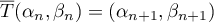 means transition from the Voronoi basis
  to the adjacent basis . Therefore, we can say that the extended Gauss measure (2.4) describes the typical behaviour of normalized Voronoi bases.
With a rational number  such that
  and it is natural to associate the lattice
  with basis matrix
  . Obviously, the map
  establishes a one-to-one correspondence between fractions of the form
  with and , and the two-dimensional primitive lattices with determinant . For
  the set of all local minima of the lattice
  coincides with the set of vertices of convex hulls of points of the lattice that lie in coordinate quadrants I and II. For
 ![$a/P=[0;a_1,\dots,a_l]\leqslant 1/2$](https://content.cld.iop.org/journals/0036-0279/70/3/483/revision1/RMS_70_3_483ieqn158.gif) the local minima have the form
the local minima have the form

where the sequences  and
and  are defined by

(For  the fraction
 ![$[0;a_1,\dots,a_l]$](https://content.cld.iop.org/journals/0036-0279/70/3/483/revision1/RMS_70_3_483ieqn162.gif) is assumed to be equal to
is assumed to be equal to  by definition.) Here the set of Voronoi bases coincides with the set of pairs
  , where
  . For
. For  the coordinates of the local minima are determined in similar fashion from the continued fraction expansion of the number
  .
.
3.2. Minkowski bases
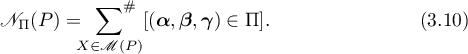
Let ![$\Pi=[0,\xi]\times [0,\eta]\subset[0,1]^2$](https://content.cld.iop.org/journals/0036-0279/70/3/483/revision1/RMS_70_3_483ieqn168.gif) , and let
, and let  denote the number of Voronoi bases
  (in all the primitive lattices with determinant ) for which the coefficients of the normalized matrix (3.2) satisfy the condition
 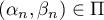 . Then (2.8) can be rewritten in the form
where
Let  denote the group generated by the following elementary transformations acting on the set of matrices:
(i) permutations of columns and multiplication of columns by  (renumbering of the basis vectors and changing their orientation);
(ii) permutations of rows and multiplication of rows by (renaming coordinate axes and changing their directions).
Two matrices are regarded as equivalent if they are taken one to the other by the action of the group .
As noted above, the purpose of this paper is to develop analytic methods that enable us to prove a three-dimensional analogue of equation (2.8). The classification of minimal triples of vectors becomes somewhat more difficult in the three-dimensional case. A complete description of minimal triples in lattices of general position is given by the following result of Minkowski.
Theorem 3.1. (Minkowski) Let  be a minimal system of a lattice
  . If the system is non-degenerate, then it is a basis of , and the matrix
  is equivalent to one of the two canonical forms
But if the system is degenerate, then  for some combination of signs, and the matrix can be reduced by the action of the group
  to the form
(In all three cases it is assumed that  and the basis matrix has diagonal dominance:
  ,
,  , and
, and  .)
.)
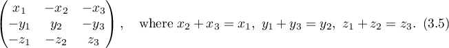
The converse is also true: a system of three vectors  with matrix equivalent to one of the matrices of the form (3.3) or (3.4) is a minimal system of the full lattice
  ; a system of vectors with matrix of the form (3.5) is a minimal system of the rank-
 lattice
  .
.
Minkowski stated this theorem without proof (see [19], [91]). A detailed proof can be found in [22], papers 109–110 (see also [95]–[98]).
In accordance with Theorem 3.1, minimal systems with matrices equivalent to (3.3) or (3.4) are called Minkowski bases of type I or II, respectively.
For reducible lattices the classification of minimal systems becomes more difficult (see [94]). But it is Minkowski bases that are of main interest, since any local minimum  can be supplemented to form a Minkowski basis by extending (in a lattice of general position that is close to the given lattice ) the parallelepiped
  along the coordinate axes.
3.3. Three-dimensional continued fractions
For an arbitrary  let
let  if
if  and
and  if
if  , and let

With each discrete set ( ) we associate the orthogonal surface
  that is defined as the boundary of the set

The Voronoi–Minkowski three-dimensional continued fraction associated with a lattice is defined as the orthogonal surface  .
.
The fact that is discrete implies that the surface  has only finitely many vertices inside any bounded set. The set of concave vertices of coincides with — the set of local minima. Corresponding to each convex vertex of is an extremal parallelepiped — a parallelepiped of the form
  , where
  are local minima that lie strictly inside three mutually perpendicular faces of . In other words, the extremal parallelepiped is characterized by the fact that its dimensions cannot be increased in such a way that it remains free of points in the set .
Example 3.2. Let consist of non-zero nodes of the lattice  , where
  ,
,  , and
, and  . Then
  , where
  and
and  . The surface is depicted in Fig. 1.

Figure 1.
Download figure:
Standard image For describing the polyhedron we define the Minkowski–Voronoi complex  as the two-dimensional complex whose vertices are the extremal parallelepipeds, whose edges are the pairs of the form
  , and whose faces are the local minima
  surrounded by chains of edges of the form

(see Fig. 2).

Figure 2. Example of the surface and the corresponding complex
Download figure:
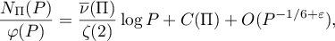
Standard image If is a set of general position, then has a more regular structure. In this case it is natural to define two mutually dual planar graphs — the Voronoi graph  and the Minkowski graph
  . The vertices, edges, and faces of the Voronoi (Minkowski) graph are assumed to be, respectively, the vertices (faces), edges, and faces (vertices) of the complex .

Figure 3. Example of a Voronoi graph
Download figure:
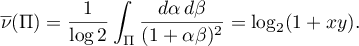
Standard image The graphs and can be depicted on the surface by using the following rules: the vertices of are peaks (convex vertices) of , the edges are pairs of convex edges of (all the vertices of  have degree ), and the faces are domains that are formed after erasing local minima and the edges going out from them (see Fig. 3); the vertices of are the local minima (concave vertices of ), each face is a triangle whose edges connect three local minima on the surface of some extremal parallelepiped (
 is a triangulation of the plane; the concave edges of can be regarded as part of the edges of ; see Fig. 4).

Figure 4. Example of a Minkowski graph
Download figure:
Standard image
Figure 5. The Voronoi graph and its canonical diagram
Download figure:
Standard image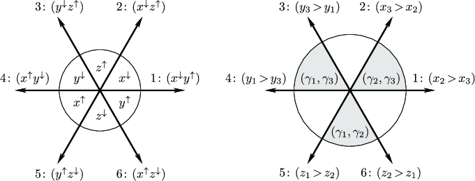
Figure 6. Geometric meaning of the directions on the canonical diagram
Download figure:
Standard image
Figure 7.
Download figure:
Standard image The edges of each of the graphs and are in a one-to-one correspondence with the saddle vertices of .
It is convenient to depict the Voronoi graph on the plane  in the form of the canonical diagram — a graph whose edges are segments of the three directions (see Fig. 5).
The canonical diagram preserves information about the mutual disposition of extremal parallelepipeds. Let  (
( ) and suppose that the matrix
  has diagonal dominance. Suppose that we pass from the extremal parallelepiped
  to the adjacent parallelepiped by moving along the canonical diagram in the `Eastern' direction (the direction in Fig. 6). Then the movement takes place along the edge with label
  , and the adjacent sector (see Fig. 6 on the right) is denoted by
  . This means that such a passage is possible only if
  , and the adjacent parallelepiped has the form
  . In particular, this implies that there exist
  types of local structure of vertices of the canonical diagram (of the two radii that cut out each of the three grey sectors, exactly one is chosen) (see Fig. 7).
The adjacent sectors in Fig. 6 on the left have labels  and
and  ; therefore, the linear dimensions of the parallelepiped compared with are smaller in the first coordinate, larger in the second, and the same in the third.
By choosing in a special way the orientation and colouring of the edges, one can introduce the structure of Schnyder trees on the Voronoi graph (see [99]). This makes it possible to depict any finite subgraph of in the form of a canonical diagram with preservation of the mutual disposition of the vertices (for any two convex vertices of the surface , their coordinates in space are connected by the same inequalities as the coordinates of the corresponding vertices of the canonical diagram on the plane ). More detailed information about Voronoi and Minkowski graphs can be found in [100].
An interesting problem is to find necessary and sufficient conditions for a graph satisfying the obvious properties of a canonical diagram to really be the canonical diagram of the Voronoi graph of some lattice. It is also unknown whether an infinite Voronoi graph can always be depicted in the form of a canonical diagram with preservation of the mutual disposition of the vertices in such way that no limit points appear. One can conjecture that this is always possible at least for the periodic Voronoi graphs corresponding to totally real cubic fields.
For a given lattice , the process of constructing the three-dimensional continued fraction of the surface consists in successively constructing elements of — the minimal triples of vectors that form the faces of  . Some triples can be degenerate (see Theorem 3.1), but such a situation cannot arise too often: faces of corresponding to degenerate triples cannot be adjacent (see [22], paper 11, Theorem 3.3). To find an initial Minkowski basis, we use methods of Voronoi (see [20], §59). At each of the next steps, we calculate the adjacent triples for a given Minkowski basis. If a triple turns out to be degenerate, then the adjacent triples are already bases (all the transition formulae can be written out explicitly; see [19], and also [22], pp. 402–405). In view of Theorem 3.1, three-dimensional continued fractions can be interpreted as a dynamical system with two-dimensional time, an invariant measure (2.13), and a phase space consisting of the matrices of
  equivalent to the Minkowski matrices (3.3) or (3.4). The algorithm for successively finding the Minkowski bases can also be applied for integer lattices, by passing to infinitesimally close lattices of general position when coordinates coincide.
The construction of three-dimensional continued fractions described above was initially proposed (in different forms) by Voronoi and Minkowski as a tool for finding fundamental units in totally real cubic fields. Corresponding to the rings of integers in such fields are lattices for which has a doubly periodic structure; thus, the problem of finding fundamental units reduces to finding minimal periods of (see [20]). For example, let  ,
,  , and
, and  be the roots of the cubic equation
  . We can choose the triple
  as a basis of the ring of integers of the field
  . Then to the fundamental units
  ,
,  there correspond two independent periods of , where is the algebraic lattice generated by the vectors
  (
( ) (see Fig. 8; the bold dots in the picture denote degenerate minimal triples of vectors).
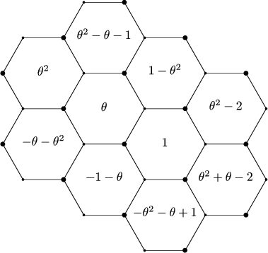
Figure 8. The Voronoi graph for the field ,
Download figure:
Standard image Figure 9 depicts the canonical diagram constructed from the triple of numbers  ,
,  ,
,  which are the roots of the cubic equation
  . A basis of the ring of integers of the field is given by , and ,
  are fundamental units.

Figure 9. The Voronoi graph for the field ,
Download figure:
Standard image The two examples above are interesting in that the numbers  and
and  are the beginning of a three-dimensional analogue of the Markov spectrum (see [101], [102], and also the isolation theorems in [103], [104]); in the classical theory of continued fractions the corresponding numbers are
For further development of the Voronoi and Minkowski algorithms see [105]–[112].
We also mention that for Voronoi–Minkowski three-dimensional continued fractions it is possible to prove an analogue of Vahlen's theorem (see [94], [95], [113]–[115]). Concerning applications of the theory of local minima see [29], [30], [116]–[122].
Information about other multidimensional generalizations of continued fractions can be found in [123].
3.4. Statement of the main result
A three-dimensional analogue of the problem of Gauss statistics for finite continued fractions is the question of the statistical properties of the Minkowski bases described in Theorem 3.1. The question of the behaviour on average of elements of Klein polyhedra reduces to the calculation of Minkowski matrices with certain additional restrictions or to the calculation of matrices with similar properties (see [27]–[30]). We confine ourselves to the consideration of Minkowski bases on totally primitive lattices (see the definition in §2.3), since this leads to a more simple and natural answer.
For a matrix of the form (1.8) let ,  , and
, and  denote the maximal absolute values of elements in the rows of :

Let  ,
,  ,
,  denote the following matrices:
In particular, if is a basis matrix of the form (3.3) or (3.4), then the matrices , , have the form
respectively, where  ,
,  ,
,  .
.
For an arbitrary matrix set  let
let  ,
,  ,
,  , and
, and  denote the following sets:

Let  be the set of Minkowski basis matrices of fixed type (I or II) with fixed signature and integer coefficients. It follows from Theorem 3.1 that in the calculation of matrices in the set it is sufficient to confine oneself to the cases when
where  ,
,  ,
,  satisfy the inequalities of Theorem 3.1.
As noted above, the main result of the paper is a three-dimensional generalization of equation (2.8), which is an asymptotic formula for the mean value of the Gauss–Kuz'min statistics of finite continued fractions. We define three-dimensional Gauss–Kuz'min statistics as follows. Let us fix a tuple of real numbers ![$(\xi_2,\xi_3,\eta_1,\eta_3, \zeta_1,\zeta_2)\in(0,1]^6$](https://content.cld.iop.org/journals/0036-0279/70/3/483/revision1/RMS_70_3_483ieqn262.gif) and consider the parallelepiped
and consider the parallelepiped

where ![$I(\xi_3)=[-\xi_3,0]$](https://content.cld.iop.org/journals/0036-0279/70/3/483/revision1/RMS_70_3_483ieqn263.gif) for matrices of type I, and
for matrices of type I, and ![$I(\xi_3)=[0,\xi_3]$](https://content.cld.iop.org/journals/0036-0279/70/3/483/revision1/RMS_70_3_483ieqn264.gif) for matrices of type II. Then the three-dimensional Gauss–Kuz'min statistics (corresponding to the matrices in of given type and signature) for a lattice
for matrices of type II. Then the three-dimensional Gauss–Kuz'min statistics (corresponding to the matrices in of given type and signature) for a lattice  are defined to be sums of the form

where  ,
,  ,
,  , and
, and  ,
,  ,
,  are found from (3.7) and (3.8). Under this approach, a three-dimensional analogue of the sum on the left-hand side of equation (2.8) is the quantity
Henceforth the symbol  means that the sum is taken over totally primitive matrices , that is, over matrices satisfying the conditions (2.9)–(2.11).
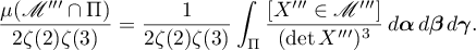
Theorem 3.3. For any positive integer and any real 

where  is a polynomial of second degree with leading coefficient
A detailed scheme of the proof of Theorem 3.3 is given in §5.3.
§ 4. Two-dimensional case as a model problem
4.1. Statement of the problem
We write Voronoi matrices in the form

Let  denote the set of all primitive Voronoi matrices:

Let and (within §4) denote the maximal absolute values of the elements in the rows of the matrix :

Here  . For a matrix
  , let
, let  and
and  denote the matrices
The corresponding sets are denoted by  and
and  :
:
Let us fix a pair of real numbers  ,
, ![$\eta\in[0,1]$](https://content.cld.iop.org/journals/0036-0279/70/3/483/revision1/RMS_70_3_483ieqn283.gif) and define the rectangle
and define the rectangle ![$\Pi=[0,\xi]\times [0,\eta]$](https://content.cld.iop.org/journals/0036-0279/70/3/483/revision1/RMS_70_3_483ieqn284.gif) . We consider the problem of calculating the quantity
. We consider the problem of calculating the quantity
equal to the number of primitive Voronoi matrices with determinant for which the coefficients of the normalized matrix belong to  . A solution to this problem is given by the following theorem.
Theorem 4.1. Let be a positive integer and a real number. Then

where

The remainder term in Theorem 4.1 is worse than the remainder term in Porter's result (1.11). This is due to the fact that the proof of Theorem 4.1 is simpler: instead of estimates of trigonometric sums by van der Corput's method, this proof uses the idea of approximating the boundaries of domains by step-functions. The proof of Theorem 3.3 (a three-dimensional analogue of Theorem 4.1) is based on the same approach. Below, all the main steps are briefly described in order to sketch the scheme of proof of the main result.
4.2. Division into cases
We divide the set of all Voronoi matrices into two parts:

Correspondingly, the quantity  can be represented in the form
  , where the definition of
  (
( ) is obtained from the definition of by imposing the additional condition
  . To prove Theorem 4.1 it suffices to verify the asymptotic formula

The proof of (4.3) for  will imply that if the non-strict inequality
  in the definition of
  is replaced by the strict inequality
  , then only the form of the constant
  changes in (4.3). The map
establishes a one-to-one correspondence between the matrices in the set  for which
  and the matrices in
  . Therefore, to prove (4.3) for
  (and thus Theorem 4.1) it suffices to verify this equation for . In what follows we assume that .
Let  denote the set of matrices
  for which
  . The sets
  and
and  are defined by analogy with and .
To verify (4.3) we first prove an asymptotic formula for  . We do this in two different ways, first by elementary considerations, and second by using estimates of Kloosterman sums.
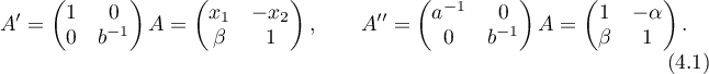
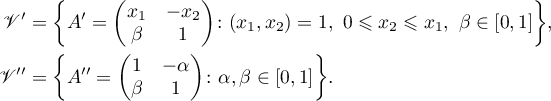
4.3. Linear parametrization of solutions
If we fix numbers and  with
with  , then we can find integers
  and
and  such that

Thus, all the solutions of the equation
with respect to the unknowns  , admit the linear parametrization
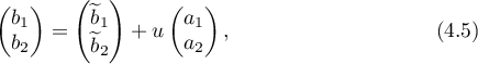
where  and
and  . It follows from the equalities

that a solution obtained by the formula (4.5) defines a primitive matrix if and only if  .
.
4.4. First variant of estimation of the remainder term
We obtain an asymptotic formula for  based on elementary considerations. It follows from the equality
 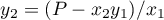 that the conditions
  and characterizing the set (recall that we consider only the case ) can be written in the form
  , where

Furthermore,

and (under the condition that  )
)

Using the linear parametrization (4.5), we find that
Passing to the variable  and using the equalities
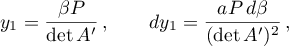
we rewrite (4.9) in the form
Summing the last equation over  and passing to the variable
  , we find that

where  .
.
Remark 4.2. Both sides of (4.9) are estimated as  . This enables us to obtain, in particular, the following asymptotic formula with a trivial estimate of the remainder:
4.5. Second variant of estimation of the remainder term
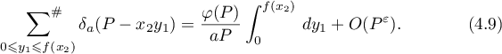
The second approach to the calculation of consists in counting the number of solutions of the congruence  that lie below the graph of some monotonic function. We approximate this domain by rectangles, and in every rectangle we reduce the problem to estimates of Kloosterman sums.


Then the asymptotic formula
holds, where
Proposition 4.3 is proved by standard methods (see, for example, Theorem 3 in [24]; a generalization to the case of an arbitrary linear function can be found in [124]). It follows from the formula (4.12) that for an arbitrary non-negative function  such that
  (
( ) for
) for  the following asymptotic formula holds:
We apply this formula to the function defined by (4.6). For this we choose a positive integer  and represent the interval
 ![$[0,a]$](https://content.cld.iop.org/journals/0036-0279/70/3/483/revision1/RMS_70_3_483ieqn331.gif) in which varies in the form
in which varies in the form
where  ,
, ![$I(0)=W_0=[0,a/r]$](https://content.cld.iop.org/journals/0036-0279/70/3/483/revision1/RMS_70_3_483ieqn333.gif) ,
,
We represent the quantity in the form
where the definition of  is obtained from the definition of by imposing the additional condition
  . By approximating on each interval
  by constant functions one can prove that

For this it is sufficient to use the formula (4.11) for  and to sum equation (4.13) over the intervals
  for
for  . By (4.7) and (4.8) we have
  on each of these intervals. The values of vary within an interval of length
  , and this leads to a remainder
  . It remains to take into account that the number of intervals is
  .
.
We sum (4.14) over and pass to the variables and :

The value ![$r=[P^{1/2}a^{-3/4}]$](https://content.cld.iop.org/journals/0036-0279/70/3/483/revision1/RMS_70_3_483ieqn344.gif) is chosen based on the relation
is chosen based on the relation  . The requirement holds under the condition that
  . As a result we obtain an asymptotic formula for with a second version of the remainder:

4.6. Estimation of the total remainder
Comparing the formulae (4.10) and (4.15), we find that it makes sense to use the first one for  and the second for
  . Thus, for the sum of all remainder terms we obtain the estimate

4.7. Calculation of the principal term
If  , then the set becomes empty. Nevertheless, we can impart a meaning to the formula (4.10) by setting
  . Under this convention, it follows from the estimate that
As noted above, the condition  , which is satisfied by the matrices in the set , is equivalent to the inequality
  . Therefore, the relations (4.10), (4.15), and (4.16) imply that

The condition  , which must be satisfied by the matrices in , is not invariant under the left action of
  . When we pass to the set
  , this condition takes the form , that is,
Thus,
Applying the relation
to the inner sum, we arrive at the required formula (4.3).
§ 5. Division into cases
In the two-dimensional case the set was divided into two subsets and which were almost the same (see §4.2). In the three-dimensional case the division has a more complicated structure and essentially uses geometric properties of Minkowski bases.
5.1. Reduced matrices
Let be a Minkowski basis matrix of the form (1.8) and let  be defined by (3.6). Then
  . Indeed, on the one hand, the obvious inequality
  holds. On the other hand,
  by Minkowski's convex body theorem. In particular, the inequality means that among the minors corresponding to the elements of any row of , there always is at least one that has maximal possible order. For example,

An important role in the arguments below will be played by division of the set of all Minkowski basis matrices into charts — subsets on which the Linnik–Skubenko reduction will be conducted. In every chart the position of the minor of maximal order (for every row) will be fixed.
Definition 5.1. Let , let  , and let be the matrix of a Minkowski basis of the form (1.8). The matrix is said to be reduced if it satisfies the following conditions.
- (1)
 .
. - (2).
- (3)The basis of the lattice is close to a minimal basis in the following sense: one of the bases , , is a Voronoi basis of .


In other words, the properties 1 and 2 mean that in a reduced matrix the corner minor and the corner element have greatest possible values with respect to the order. The property 3 means that the matrix can also be reconstructed from the lattice with basis  ,
,  almost uniquely: the number of Voronoi bases in a lattice with determinant , like the length of the continued fraction expansion of the number
  , can be estimated as
  , and therefore the number of possible matrices for the given lattice is bounded by a quantity .
We denote by  the elements of the group permuting the coefficients of the matrix (and preserving the diagonal dominance of ).
Lemma 5.2. The set can be partitioned into finitely many subsets in such a way that:
(i) every set of the partition is defined by a finite set of inequalities that are invariant under the left action of ;
(ii) if  is one of the sets of the partition, then for any
  at least one of the sets
  or
or  consists of reduced matrices.
Proof. By Theorem 3.1, it is sufficient to construct a required partition for the sets (3.3) and (3.4). In each of them we add the additional partition by all hyperplanes of the form  ,
,  ,
,  (
( ). Consider an arbitrary set in the resulting partition. If it consists of matrices of type I, then all its elements satisfy the conditions 1–3 (the matrix defines a Voronoi basis, since
  ).
).
Suppose that the set under consideration consists of matrices of type II. After the rows of the matrix are ordered by increase of maximal elements, there arise three variants of sign arrangements. Besides the case (3.4), there are also the following two possible cases:
In the matrices (3.4) and (5.1), the element is negative. Hence, as for matrices of type I, we have  and the basis
  is a Voronoi basis. For the matrices (5.2) we implement in addition the subpartition by the planes
  and
and  and consider two cases:
- 1) and ( or (, ));
- 2), , .


In the first case,  , and for
  we can choose as a Voronoi basis the pair
  with the matrix
  , while for
  we can choose the pair
  with the matrix
  .
.
In the second case, we transpose the second and third columns in :
If the condition  holds in the matrix
  , then the basis of
  consisting of the vectors
  and
and  is a Voronoi basis and
  . In the remaining case (
 ,
,  ) we can choose as a Voronoi basis the pair
  with the matrix
  . Here
  .
. 
Thus, with each matrix we can associate a Voronoi basis of the lattice , and to each Voronoi basis there correspond at most four matrices .
Remark 5.3. It suffices to prove Theorem 3.3 after replacing in its statement (and in the definition (3.10) of the quantity  ) the set by an arbitrary set of the partition constructed in Lemma 5.2. Then the set can be represented in the form
where  , and each of the sets
  consists of reduced matrices satisfying the conditions
  (in the definition of , the non-strict inequalities between , , and can be replaced by strict inequalities, so that the sets
  are pairwise disjoint).
Remark 5.4. The three-dimensional Gauss measure is invariant under the left action of . In particular, for  ,
,  ,
,  , and
, and  we have
Thus, the measure of the set  is independent of whether the second and third columns of the matrix were transposed or not.
Remarks 5.3 and 5.4 imply that to prove Theorem 3.3 it suffices to verify the following assertion.
Theorem 5.5. Let be one of the sets of the partition (5.3) and let be the parallelepiped defined by equation (3.9). Then

where  is a polynomial of second degree with leading coefficient

To simplify the exposition, we conduct the proof of Theorem 5.5 under the assumption that all the parameters  defining the dimensions of are equal to 1. In the general case the arguments will be the same.
5.2. Properties of the constructed partition
Lemma 5.6. Suppose that is a reduced matrix. Then
Proof. The assertion of the lemma follows from the inequalities  and
and  and the property 2 of reduced matrices.
Lemma 5.7. The partition constructed in Lemma 5.2 has the following additional properties: any of the sets  is defined by finitely many inequalities of the form
  (
( ) each of which acts over the corresponding domain
  . Furthermore,
  and
and

where  .
.
Proof. Consider Minkowski matrices of type I. Obviously, the estimate always holds, since  for reduced matrices (see Lemma 5.6). We consider successively all the functions that can define the limits of variation of
  for the matrices of the form (3.3) with . These are the functions
  (
( ) that are defined, respectively, by the conditions
  ,
,  ,
,  (arising in the initial partition of the set ), and
  (the part of the boundary appearing because of the inequality
  ). For the first function
  we have
The other functions are found from the equation :
(If a function  , where , defines the boundary of the domain of variation of
  , then, as noted above, , and therefore the denominator
  in such cases is non-zero.) If
  , then
For all the functions under consideration we have
Therefore, to verify the assertion of the lemma it is sufficient to show that  . For
. For  and
and  this is obvious, and for
  it follows from the inequalities on the elements of the Minkowski matrix:

(for  this follows from the inequality
  , for it follows from the inequality
  , but for
  the function cannot define the boundary of the domain of variation of , since then the inequality
  would hold inside this domain, which contradicts the condition defining ).
For matrices of type II, the only difference in the proof of the estimates (5.6) is the need to consider the function  defined by the condition
  . For this function the conditions (5.6) are verified in the same way as for the other functions.
5.3. Scheme of proof of the main result
To prove (5.4) we represent the set  in the form
where is the set of matrices  in which the values of the corner element
  and the corner minor
  are fixed. Then

In the last equation it is assumed that in the summation over ,  , ,
, ,  ,
,  , the values of and
  are determined by the equations
  and , respectively.
In the process of the proof we will pass successively (in various orders) from summation over the variables , , , , , to integration over the variables  ,
,  ,
,  . In the end this will enable us to transform the sum in (5.7) into the integral in (5.5).
We define the parameters  and
and  by
by  and
and  . In addition we divide the domain

in which the pairs  vary into three parts depending on the values of and (see Fig. 10).

Figure 10. Partition of the domain of variation of the parameters and
Download figure:
Standard image We prove the asymptotic formulae for  in three different ways, depending on which of the domains
  () the pair belongs to.
1. For small values of and (that is, for  ), equation (1.2) is first solved as a linear equation with respect to , , (see §6). The solutions are counted by elementary considerations. A reduction is performed to a two- dimensional problem, which is solved by the methods of §4.
2. If the values of , , are commensurable (that is, for  ), then the matrix
  is fixed and equation (1.2) can be solved with respect to the unknowns , , , , (see §7). The solutions are counted by using a non-linear Linnik–Skubenko parametrization and estimates of Kloosterman sums. Again a reduction is performed to a two-dimensional problem, which is also solved by using the methods of §4.
3. In the remaining case, when is small while and are large (that is,  ), equation (1.2) is solved with respect to the unknowns , , , (see §8). The reduction to a two-dimensional problem is effected by using a special version of the Linnik–Skubenko reduction which preserves the value of , and this two-dimensional problem is solved by elementary methods.
Correspondingly, the quantity  is represented in the form

where
For each case we indicate the order of the transitions from summation to integration and the assertions in which these transitions are effected.
1.  , Lemmas 6.2, 6.3, and 6.4; , Lemma 6.7; , Lemma 6.9;
  , Lemma 9.13; , Proposition 9.14.
2. 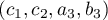 , Theorem 7.1 and Corollary 7.3;
  , Proposition 7.7; , Proposition 9.12.
3.  , Theorem 8.1 and Corollary 8.2; , Proposition 8.3; , Lemma 9.13; , Proposition 9.14.
After this, the three results obtained are substituted into equation (5.8). The last transition, from summation to integration with respect to the variable , is implemented in the proof of Theorem 5.5.
After the transition to matrices in which some coefficients become real numbers, the symbol will mean that instead of the total primitivity conditions (2.9)–(2.11) only those necessary restrictions hold that make sense (that is, those in which only integers occur):
5.4. Different versions of Kloosterman sums
For the Kloosterman sums (1.6) we know the estimate

( is the number of divisors of ), proved by Weil [125] for prime and extended to arbitrary by Estermann [126].
The trigonometric sums (1.5) are responsible for the distribution of the solutions of equation (1.3) (and the equivalent congruence (1.4)). For these sums it is convenient to use the estimate

(see [44], Lemma 1), which generalizes the inequality (5.10).
As noted above, in the proof of the main result of this paper the reduction to the two-dimensional case is performed in three different ways. In the first two cases it is necessary to study solutions of the equation (1.3) (the congruence (1.4)) under the additional conditions  or
or  . The corresponding trigonometric sums are defined by

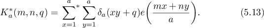
Estimation of the sums (5.12) and (5.13) reduces to the estimate (5.11) (see [24], Lemma 1–3). In both cases this makes it possible to prove the uniform distribution of the solutions of the congruence  with the corresponding restrictions (see Propositions 6.8 and 7.4 below). For brevity we use the notation
§ 6. First variant of estimation of the remainder
In this section the reduction to the two-dimensional case is performed by elementary considerations. For the two-dimensional case similar arguments were described in §§4.3 and 4.4. In the transition to integration in the second row of the matrix , standard `two-dimensional' methods are used, based on estimates of Kloosterman sums (see §4.5).
6.1. Linear parametrization of solutions
Lemma 6.1. A matrix with determinant  can be supplemented to form a matrix
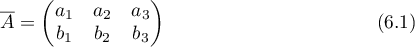
satisfying the condition
if and only if  .
.
For an arbitrary matrix  satisfying the condition (6.2) there are integers , , such that
See the proof in [23].
Lemma 6.2. If the matrix (6.1) satisfies the condition (6.2) and  is a particular solution of equation (6.3), then the following assertions hold.
(i) All the solutions of the equation
with respect to the unknowns  have the form
(ii) The formula (6.5) produces different solutions  for different pairs
  .
.
(iii) A solution obtained by the formula (6.5) defines a totally primitive matrix (1.8) if and only if  .
.
Proof. (i) An arbitrary integer vector  can be represented as a linear combination of the vectors
  ,
,  , and
, and  with integer coefficients. It follows from (6.4) that the coefficient of
  must be equal to . This proves that representation in the form (6.5) is possible.
(ii) It follows from condition (6.2) that the vectors and are linearly independent. Therefore, different solutions correspond to different pairs .
(iii) The last assertion of the lemma is verified using the formulae (6.5) and (6.2):
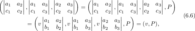
Thus, the matrix is totally primitive if and only if .
Suppose that is a planar domain with rectifiable boundary. Let  denote the area of this domain, let
  be its perimeter, and let
  be the number of points of the lattice lying inside . For a convex domain Jarnik's inequality is known:

For an arbitrary simply connected planar domain with rectifiable boundary we have

(see, for example, [67], Lemma 1).
Lemma 6.3. Let be a positive integer, let be a simply connected planar domain with rectifiable boundary such that  , and let
Then
Proof. By the Möbius inversion formula,
The required asymptotic formula is obtained if in the inner sum we perform the change of variables  ,
,  , use the inequality (6.8) in the new variables
  ,
,  , and estimate the perimeter of the diminished copy of the domain as
  :
:
6.2. Transition to integration in the third row
We consider the set of matrices  for which the matrix
  is fixed. Since
  , the value of is uniquely expressible in terms of and . Therefore, any conditions imposed on the variables can be written in the form
  .
.
Lemma 6.4. Suppose that  satisfies the condition (6.2), is a convex domain, and
Then

Proof. By construction the set consists of matrices of the form (3.3), (3.4), (5.1), or (5.2). Hence, the variables must satisfy some conditions in the following list:

Thus, the domain of variation of the variables  is contained in a convex polygon with linear dimensions estimated as
  by Lemma 5.6. It follows from equation (6.5) that the linear dimensions of the corresponding polygon on the plane
  are
are  . By Lemma 6.3,
Corollary 6.5. Assume the hypotheses of Lemma 6.4. Then
Furthermore, for fixed  and
and 
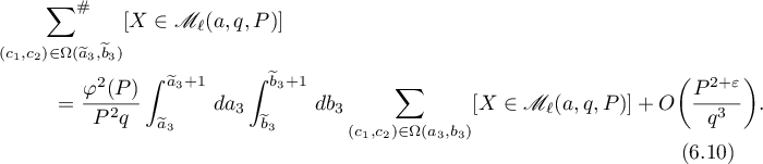
Proof. To verify the estimate (6.9) it suffices to use a trivial estimate for the integral in Lemma 6.4. Equation (6.10) follows from the fact that every term in it is  .
.
6.3. Transition to integration in the second row
By the norm of a function we always mean the  -norm.
Lemma 6.6. Let and  be positive integers with
  . Suppose that a function on an interval
  has finitely many monotonicity parts. Then the following asymptotic formulae hold:
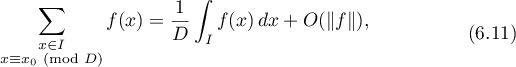
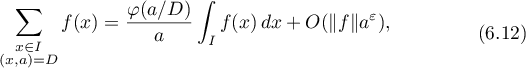
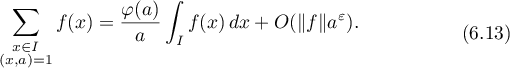
See the proof in [24], Lemma 4.
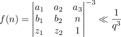
for all in an interval . Then for the sum
the following asymptotic formula holds:
Proof. Suppose that the matrix can be reduced to the form  by elementary transformations of columns. Then the condition (6.2) is equivalent to the equality
Since  , we have
  , and (6.14) means that
  . Therefore,

It follows from the condition  that
that  . By the hypothesis of the lemma, , and therefore
  . Furthermore,
  . Thus, it follows from the relations
  and
and  that
that  . For the congruence
  is equivalent to the condition
  , where
  . To complete the proof of the lemma it remains to use (6.11):
If  , then every interval
  contains exactly one solution of the congruence with respect to the unknown
  . Hence, for an arbitrary function
  defined on the rectangle
  , a natural approximation for the sum
is given by the sum
Proposition 6.8. Let be a non-negative function and suppose that for any with  the inequality
  defines in a rectangle
 ![$I=[0,a]\times [0,Z_2]$](https://content.cld.iop.org/journals/0036-0279/70/3/483/revision1/RMS_70_3_483ieqn546.gif) (where
(where  ) the domain
  , and the number of monotonicity parts for all the functions
  is bounded by an absolute constant. Then

See the proof in [24], Theorem 4.
Lemma 6.9. Suppose that and  . Then the sum
satisfies the asymptotic formula
Proof. We transform the indicated sum, introducing the variables  ,
,  , and
, and  (where
  is not necessarily an integer):
We get rid of the condition  by using the Möbius function:
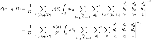
where  ,
,  , and
, and  . We apply Proposition 6.8 to the inner double sum. By the hypothesis of the lemma,
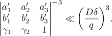
Furthermore, the function  implicitly defined by the equations
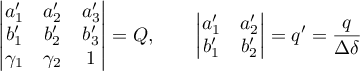
can be reduced to the form
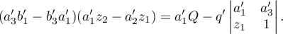
Therefore, the graph of consists of finitely many monotonicity parts, and Proposition 6.8 is indeed applicable. Thus,
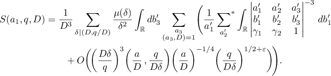
We sum the remainders that have appeared. The variable  varies in an interval of length
  , and the variable in an interval of length
  . Thus, the sum of the remainders can be estimated by the sum

We transform the sum of the principal terms, passing to the variables  and
and  :
:
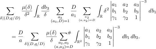
After this it remains to pass to the variables  and
and  , where
 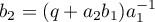 . Since
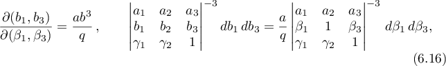
we obtain the required principal term
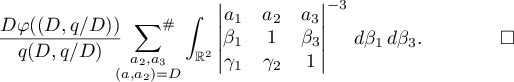
Proposition 6.10. Suppose that  . Then for the quantity defined by (5.7) the following asymptotic formula holds:
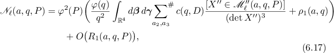
where  ,
, 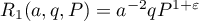 ,
,


Proof. It follows from the inequality (5.11) that

We transform the sum , using Lemma 6.4 and the estimate (6.20):
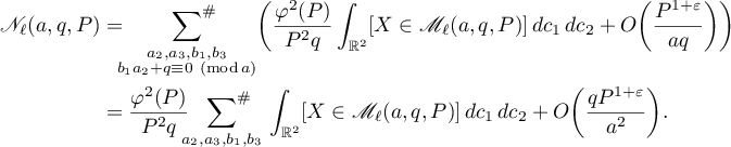
In the double integral we pass to the variables  and
and  . Since
  , we have
Therefore,
Using Lemma 6.7, we replace the summation over the variable by an integration:
By Lemma 6.9 we arrive at the following equation, which is equivalent to the formula (6.17):
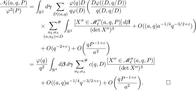
§ 7. Second variant of estimation of the remainder
Let  and
and  denote successive minima of a two-dimensional lattice , that is, is the length of a shortest non-zero vector
  , and is the length of a shortest vector
  that is linearly independent of
  . Let
. Let  denote the lattice consisting of solutions of the system of congruences

and let

Theorem 7.1. Suppose that the matrix is fixed, , , and the matrix has the form (1.8). Then for any parallelepiped

with dimensions satisfying the conditions  and
and  ,
,
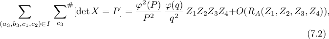
where
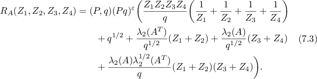
See the proof in [23].
Remark. Theorem 7.1 is a variant of Lemma 7 in [8]. But in [8] the contribution of the summands containing  and
and  in the remainder term was not taken into account. Further arguments show that it is these summands that make the main contribution to the final remainder (see the choice of the parameters
  and in the proof of Proposition 9.8). Here the estimate
  is used, which is valid only on average with respect to .
Corollary 7.3. Suppose that the hypotheses of Theorem 7.1 hold, the dimensions of the parallelepiped

satisfy the inequalities  and
and  , and for
  the values of a non-negative function
  vary within the interval
  , where
  . Then
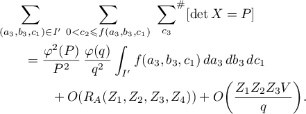
Proof. Replacing in the second sum by  and
and  , we obtain, respectively, a lower and an upper estimate of the sum being calculated. Applying Theorem 7.1 and using the estimate

we arrive at the assertion of the corollary.
Proposition 7.4. Let be a positive integer, let be an integer, let  , where
  , and let
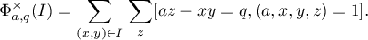
Then

where

See the proof in [24], Theorem 2.
Corollary 7.5. Suppose that the hypotheses of Proposition 7.4 hold and that for  the values of a function
  are contained in the segment
 ![$[Z_3,Z_3+V]$](https://content.cld.iop.org/journals/0036-0279/70/3/483/revision1/RMS_70_3_483ieqn598.gif) , where
, where  and
and  . Then
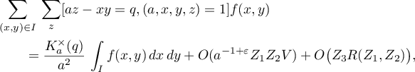
where  is defined by (7.5).
Proof. Replacing in this sum by  and
and  , we obtain, respectively, a lower and an upper estimate for this sum. Using Proposition 7.4, the estimates (6.20), and

we arrive at the assertion of the corollary.
Corollary 7.6. Suppose that the hypotheses of Proposition 7.4 hold and for  the values of a function are contained in a segment
 ![$[0,Z_3]$](https://content.cld.iop.org/journals/0036-0279/70/3/483/revision1/RMS_70_3_483ieqn605.gif) . Then
. Then
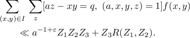
Proposition 7.7. For any positive integers 
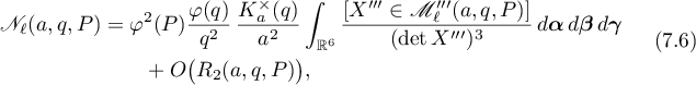
where

and the remainders and  are determined by (7.5) and (7.3), respectively.
Remark 7.8. For the parameter defined in (7.1), we use the trivial estimate  . Using the analogous estimate for does not enable us to single out the principal term in Theorem 3.3. In what follows we will prove (see §9.1) that, on average with respect to , the upper estimate
  holds and is close to the lower estimate. This is the reason for keeping the summation over and in the remainder term
  . A similar situation arises in Proposition 8.3.
Proof. of Proposition 7.7 The transition from (7.10) to (7.11) will be realized in two stages. First, by using Corollary 7.3 we pass from summation to integration with respect to the variables , , , , and then by using Corollary 7.5 we pass from summation to integration with respect to the variables , .
The intervals

(their lengths were estimated in Lemma 5.6) in which the respective variables , , vary are divided into equal intervals, and the intervals  (
( ;
;  ,
,  ) in which , vary are divided into
  equal intervals:
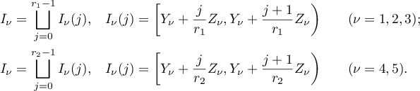
We define a function

It follows from the estimates  that the rectangle
  can be represented in the form
 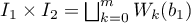 , where and
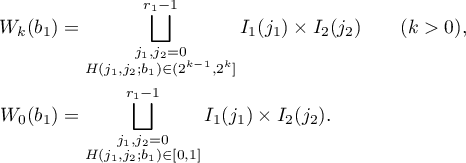
Correspondingly, we write the sum in the form
where

Then Proposition 7.7 will be proved if we show that
where

Indeed, it follows from (7.11) and (7.9) that
Thus, to obtain (7.6) it remains to pass from the variables  to the variables
  using the relations (6.21), (6.16), and
We now estimate the number of rectangles of the partition
in each of the sets  . If
. If  , then there is a point
  for which
  . Since , this inequality defines a strip of width
  on the plane
  (in the direction of the
  -axis). Therefore, above each point of the
  -axis there are
  rectangles of the partition (7.13) that have common points with this strip. Consequently, the set consists of
  rectangles of the partition.
We represent the sum  in the form

where
We now prove the asymptotic formula
where  is defined by (7.12).
We note that the number of points in each of the parallelepipeds of the partition (7.13) can be estimated as  . Thus, it follows from equation (6.10) (see Corollary 6.5) that for any rectangle
  we can use the following formula with a trivial estimate for the remainder term:
For equation (7.15) follows from (7.16). Hence, we assume that  in what follows.
For fixed and the pair of variables  can vary inside some rectangle
  , by the definition of the Minkowski matrices (3.3) and (3.4). Let
  denote the domain consisting of those rectangles of the partition (7.13) that are completely contained in , and let
  be the domain consisting of the rectangles of (7.13) that have common points with the boundary of . Obviously, consists of
  rectangles of (7.13), and by (7.16) we have
Thus, to prove (7.15) it suffices to verify that
where  .
.
Let us fix an arbitrary rectangle 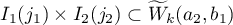 . We apply Corollary 7.3 on each of the parallelepipeds
 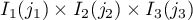 . Since
  (), we have
  , and by Lemma 5.7 each of the functions defining the boundary of the set
  satisfies the estimates

Therefore, on each of the parallelepipeds the values of the function (under the condition that its graph defines the boundary) are contained in an interval of length  . By Corollary 7.3,
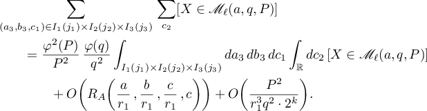
We arrive at (7.17) by summing the last equality over  and over the rectangles (the number of which is ). Thus, (7.15) is also proved.
Substituting (7.15) into (7.14), we get that to prove the main formula (7.6) it suffices to verify that
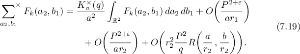
We note that

and therefore  always satisfies the trivial estimate
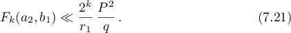
Hence, by Corollary 7.6, in each of the rectangles of the partition
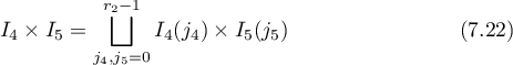
we can apply the formula
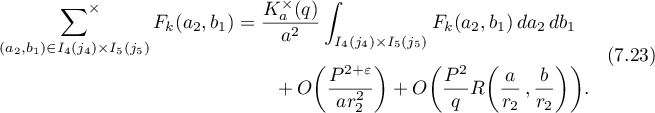
The boundary of the domain of variation of the pair of variables is determined by the conditions  and
and  (where
 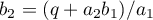 ) and therefore consists of parts of the graphs of the functions

Let  denote the domain consisting of those rectangles of the partition (7.22) that are completely contained in the domain of variation of , and let
  be the domain consisting of those rectangles of (7.22) that intersect the boundary of the domain of variation of . It follows from the monotonicity of the function (7.24) that consists of
  rectangles of (7.22). Using the formula (7.23) in each of them, we get that
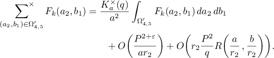
Therefore, to prove (7.19) it is sufficient to verify the asymptotic formula
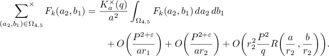
This equation in turn is a consequence of the fact that for any rectangle 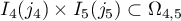 we have
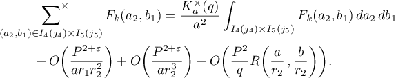
The last relation follows from Corollary 7.5 under the condition that the values of vary within an interval of length
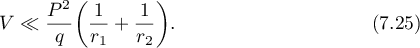
We now verify this condition.
Since , it follows from Lemma 5.7 that each of the functions defining the boundary of the domain (for  ) satisfies estimates analogous to (7.18):
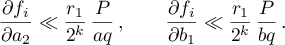
Hence, for  the area of the domain can vary within an interval of length
 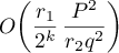 . This implies that the values of can vary in an interval of length
which agrees with the estimate (7.25).
The values of can vary also because the domain  changes. Suppose that different domains correspond to different values of . Assume that
  and
and  . For example, suppose that
  , that is,

where the function  is defined by (7.8). The values of for fixed
  and different
  can differ by
  . Moreover,
  . Therefore, for a fixed
  the number of indices
  for which the conditions (7.26) can hold can be estimated as
  . Thus, the areas of the figures and
  differ by at most
This fact and the estimate (7.20) imply that the values of can then vary in an interval of length
which again agrees with the estimate (7.25).
§ 8. Third variant of estimation of the remainder
Theorem 8.1. Suppose that a matrix and a coefficient are fixed, , ,  , , and a matrix has the form (1.8). Then any parallelepiped

with  and satisfies
where
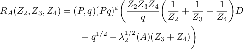
and is defined in (7.1).
See the proof in [23].
Corollary 8.2. Suppose that the hypotheses of Theorem 8.1 hold, the dimensions of the rectangle

satisfy the inequalities and , and for  the values of a non-negative function
  vary within an interval , where . Then
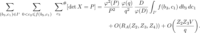
The proof is similar to the proof of Corollary 7.3.
Proposition 8.3. Let be a positive integer such that  . Then the sum in (5.7) satisfies the asymptotic formula
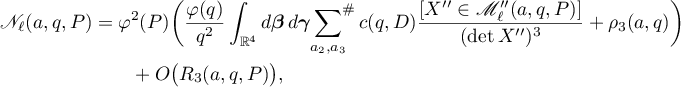
where  is defined by (6.18),
 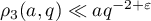 ,
,
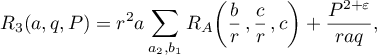
and  is the remainder in Theorem 8.1.
Proof. The first part of the proof in essence repeats the proof of Proposition 7.7.
The intervals  and
and  (see (7.7)) in which the respective variables and vary are divided into equal intervals:

We define a function

Let the interval  be represented as
  , where ,
We write the sum  in the form
where
Let us now verify the asymptotic formula
To this end we first estimate the number of intervals  contained in each of the sets . If
  , then there exists a point
  for which the inequality
holds. Since , this inequality defines a segment of length  on the -axis. Therefore, there exist intervals which have common points with this segment, that is, the set consists of intervals of the partition.
It follows from (6.10) that for any interval we have the following asymptotic formula with a trivial estimate of the remainder term:
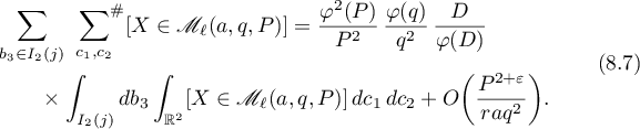
For equation (8.5) follows from (8.7). Hence, in what follows we assume that .
Equation (8.5) will be proved if for any interval we show that
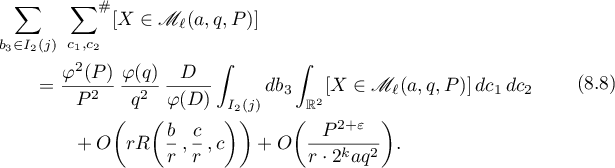
(For the intervals that intersect only partially, it suffices to use (8.7).)
If  , then
  . Therefore, it follows from the conditions (5.6) that for each of the functions whose graphs define the boundary of we have the estimates
Hence, on each of the rectangles  the values of the functions (under the condition that the corresponding part of the graph defines the boundary) are contained in an interval of length
  . On each of the parallelepipeds
  with
with 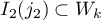 we use Corollary 8.2:
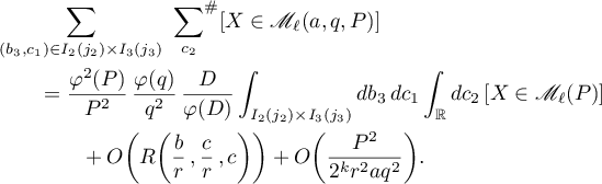
Summing the resulting equation over , we arrive at (8.8). Thus, (8.5) is proved.
The further steps will be different from the proof of Proposition 7.7.
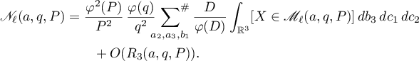
Using (6.21), we pass to the variables  :
:
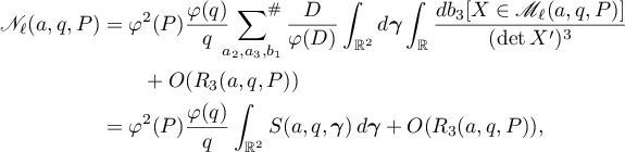
where

To prove the proposition it remains to verify that the sum  satisfies the asymptotic formula

where is defined by (6.18).
Suppose that the values of , , ,  , and
, and  are fixed and consider the sum
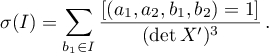
Let  be a particular solution of the equation
  . Then
and all the solutions of the equation with respect to the unknowns  can be written in the form

Since  , we have

Therefore,
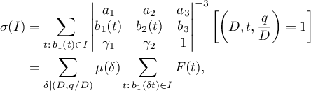
where
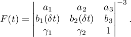
This function has finitely many monotonicity parts and satisfies the estimate  . By Lemma 6.6,
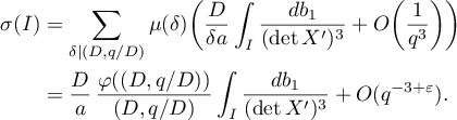
The formula for  thus obtained lets us replace the summation over the variable in (8.9) by integration. Using the definition (6.18) of , we find that

Passing from the variables  to the variables
  and using (6.16), we obtain the required formula (8.10). Proposition 8.3 is proved.
§ 9. Completion of the proof of the main result
9.1. On reduced bases in planar lattices
Lemma 9.1. Let  be a positive integer, let
  and
and  be real numbers, and let
  be a continuously differentiable function defined on the segment
 ![$[\lambda_1,\lambda_Q]$](https://content.cld.iop.org/journals/0036-0279/70/3/483/revision1/RMS_70_3_483ieqn711.gif) . Then
. Then
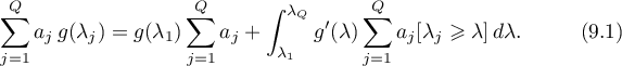
Proof. To verify the assertion of the lemma it suffices to transform the integral on the right-hand side of (9.1):
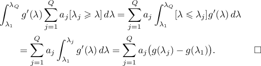
Corollary 9.2. Suppose that the hypotheses of Lemma 9.1 hold and  . Then
Lemma 9.3. Let  be a real number. Then the number of lattices
  such that
  and
and  can be estimated as
  .
.
Proof. Since  , the assertion of the lemma obviously holds for
  . Thus, in what follows we assume that
  . Let be a reduced basis of the lattice with determinant (that is, is a shortest vector of the lattice, and the projection of
  onto lies between
  and
and  ). Then it follows from the inequality
  that
that  . For a fixed vector
  the endpoint of the vector
  must lie on the straight line
  and satisfy the condition
  . Therefore, the vector can be chosen in
  ways. Thus,
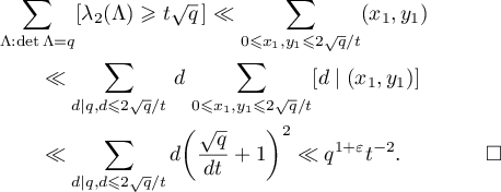
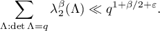
Proof. We use Corollary 9.2, setting  . As
. As  we choose the numbers taken for all lattices with determinant and ordered in ascending order. Furthermore,
 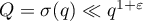 and
and  (we can always choose a vector with length of order
  and supplement it to form a reduced basis with determinant ). Hence,
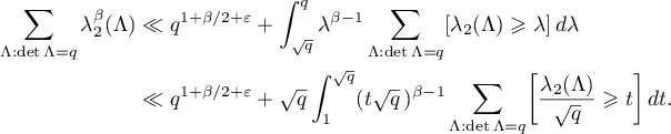
Substituting the estimate in Lemma 9.3 into the last integral, we arrive at the assertion of the lemma.
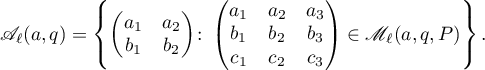
Then
By the property 3 of reduced matrices, to each term in the inner sum there corresponds some Voronoi basis of the lattice , and to each Voronoi basis there correspond at most four matrices . Consequently, the inner sum can be estimated up to a constant by the number of minimal bases, that is,
Estimating the remaining sum by Lemma 9.4, we arrive at the assertion of the corollary.
Corollary 9.6. Suppose that  ,
,  , and
, and  is an arbitrary real number. Then

Proof. The required estimate is obtained from Corollary 9.5 by using the Abel transformation

Setting  and
and ![$g(a)=\sum_{a_2,b_1}\lambda_2^\beta(A)[A\in\mathscr{A}_\ell(a,q)]$](https://content.cld.iop.org/journals/0036-0279/70/3/483/revision1/RMS_70_3_483ieqn740.gif) , we get that
, we get that
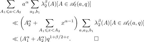
9.2. Estimation of the remainder term
Lemma 9.7. Let be a positive integer, and let  be real numbers with
  . Then
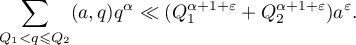

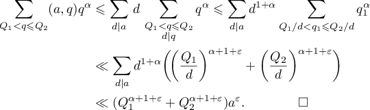
Proposition 9.8. The following estimates hold:
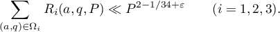
Proof. We sum the remainder 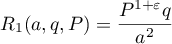 (see Proposition 6.10) over the points :
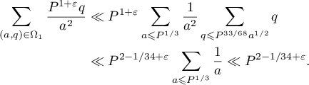
Let us estimate the sum of the remainders . By Proposition 7.7,
We choose the values of the parameters  based on the equations
assuming that  :
:
(Note that the estimates hold in the domain  , and therefore Proposition 7.7 is indeed applicable.) Then it follows from the inequality
 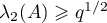 that for
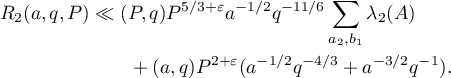
We estimate the sum of each of the terms over the pairs . For the first term,
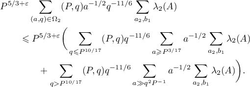
Applying Corollary 9.6 and Lemma 9.7 to the inner sums, we arrive at the required estimate:

We sum the remaining part of the remainder . The required estimate also is verified by using Lemma 9.7:
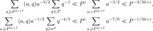
Consider the third remainder (see Proposition 8.3):
We choose the value  based on the equation
again assuming that . For this choice of and for we have
Applying Corollary 9.6 and Lemma 9.7 successively, we find that
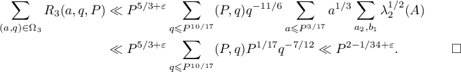
9.3. Auxiliary assertions
Along with the Euler function  , we use the functions


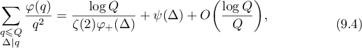
where  is an absolute constant,
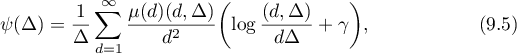
and is the Euler constant.
Proof. We verify equation (9.2). Expressing  in terms of the Möbius function, we arrive at the relations
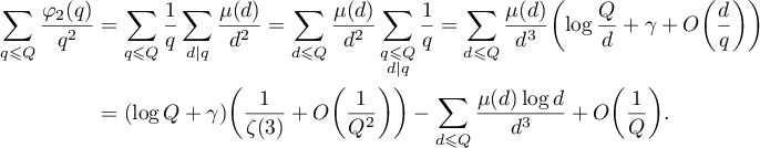
To calculate the resulting sum it is sufficient to use the fact that
and in particular,
We transform the second sum:
Using the equation
where is the first Stieltjes constant (see [127], §2.21), we find that

Setting
we obtain the second formula of the lemma.
See the proof of (9.4) in [24], Lemma 9.
Lemma 9.10. Let be a positive integer and let be defined by (6.18). Then the sum
satisfies the asymptotic formula
Proof. Setting  , we obtain for this sum the representation
We transform the sum obtained, introducing the parameters  ,
,  , and
, and  :
:
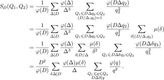
We apply equation (9.4) to the inner sum:
Substituting the equation (see [24], Lemma 8)
into the last formula, we arrive at the assertion of the lemma.
9.4. Calculation of the principal term
To complete the proof of Theorem 5.5 it remains to pass to integration with respect to the variables in the first row of the matrix . First we need to sum over the variable .
The conditions satisfied by the matrices are not invariant under the left action of . We express and from the equalities
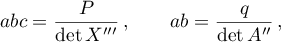
where  . Then after passing to the set
  , the inequalities take the form
Therefore, for given coefficients of the matrix , for each the domain  in which and can vary is defined by

Remark 9.11. As in the two-dimensional case (see §4.7), it is natural to extend by zero the values of the functions  for those pairs for which the sets are empty. Thus, we assume that the values are defined for all positive integers and .
Proposition 9.12. The quantity  defined by (5.9) satisfies the asymptotic formula
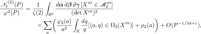
where  .
.
Proof. By Propositions 7.7 and 9.8 we have

where
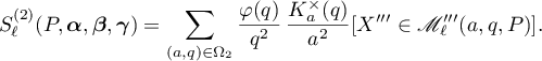
The set  is obtained from by discarding the conditions (9.7) while keeping the remaining (invariant) inequalities. Therefore,

and

We apply the relation
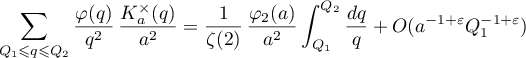
(see [24], Corollary 3) to the sum obtained above. The lower limit of summation  satisfies the estimate
  . Thus,

Substituting the last formula into (9.8), we arrive at the required equality.
Lemma 9.13. Suppose that ![$\Omega\subset[-a,a]^2$](https://content.cld.iop.org/journals/0036-0279/70/3/483/revision1/RMS_70_3_483ieqn767.gif) and the boundary of the domain has length . Then the sum
and the boundary of the domain has length . Then the sum
satisfies the asymptotic formula
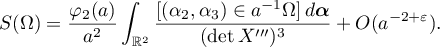
Proof. We get rid of the coprimeness condition by using the Möbius function:
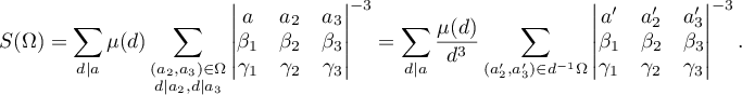
Let
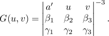
Then
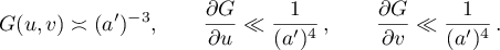
Consequently,
The number of unit squares intersected by the boundary of the domain  is
is  . In each of these squares, we can use the following formula with a trivial estimate of the remainder term:

Thus,
where  .
.
Proof. By Propositions 6.10, 8.3, and 9.8 we have
where
It follows from equation (9.9) that

We apply Lemma 9.10 to the sum over :
By Lemma 9.7,
Therefore,
Using Lemma 9.13, we arrive at the asymptotic formula
Furthermore, by Lemma 9.7 we have


Substituting (9.11), (9.12), and (9.13) into (9.10), we arrive at the required equality.
Corollary 9.15. Asymptotically,
where  .
.
For the proof it is sufficient to substitute the asymptotic formulae in Propositions 9.12 and 9.14 into (5.8).
Proof. of Theorem 5.5 Since
it follows by Corollary 9.15 that
We transform the integral with respect to the variable :
Substituting the resulting expression into the formula for and using (9.2) and (9.3), we arrive at the assertion of the theorem.