


ABSTRACT
We present the final nine-year maps and basic results from the Wilkinson Microwave Anisotropy Probe (WMAP) mission. The full nine-year analysis of the time-ordered data provides updated characterizations and calibrations of the experiment. We also provide new nine-year full sky temperature maps that were processed to reduce the asymmetry of the effective beams. Temperature and polarization sky maps are examined to separate cosmic microwave background (CMB) anisotropy from foreground emission, and both types of signals are analyzed in detail. We provide new point source catalogs as well as new diffuse and point source foreground masks. An updated template-removal process is used for cosmological analysis; new foreground fits are performed, and new foreground-reduced CMB maps are presented. We now implement an optimal C−1 weighting to compute the temperature angular power spectrum. The WMAP mission has resulted in a highly constrained ΛCDM cosmological model with precise and accurate parameters in agreement with a host of other cosmological measurements. When WMAP data are combined with finer scale CMB, baryon acoustic oscillation, and Hubble constant measurements, we find that big bang nucleosynthesis is well supported and there is no compelling evidence for a non-standard number of neutrino species (Neff = 3.84 ± 0.40). The model fit also implies that the age of the universe is t0 = 13.772 ± 0.059 Gyr, and the fit Hubble constant is H0 = 69.32 ± 0.80 km s−1 Mpc−1. Inflation is also supported: the fluctuations are adiabatic, with Gaussian random phases; the detection of a deviation of the scalar spectral index from unity, reported earlier by the WMAP team, now has high statistical significance (ns = 0.9608 ± 0.0080); and the universe is close to flat/Euclidean ( ). Overall, the WMAP mission has resulted in a reduction of the cosmological parameter volume by a factor of 68,000 for the standard six-parameter ΛCDM model, based on CMB data alone. For a model including tensors, the allowed seven-parameter volume has been reduced by a factor 117,000. Other cosmological observations are in accord with the CMB predictions, and the combined data reduces the cosmological parameter volume even further. With no significant anomalies and an adequate goodness of fit, the inflationary flat ΛCDM model and its precise and accurate parameters rooted in WMAP data stands as the standard model of cosmology.
Export citation and abstract BibTeX RIS
1. INTRODUCTION
Since its discovery in 1965, the cosmic microwave background (CMB) has played a central role in cosmology. The discovery of the CMB (Penzias & Wilson 1965) confirmed a major prediction of the big bang theory and was difficult to reconcile with the steady state theory. The precision measurement of the CMB spectrum by NASA's Cosmic Background Explorer (COBE) mission (Mather et al. 1990, 1994) confirmed the predicted CMB blackbody spectrum, which results from thermal equilibrium between matter and radiation in the hot, dense early universe. The COBE detection of CMB anisotropy (Smoot et al. 1992; Bennett et al. 1992; Kogut et al. 1992; Wright et al. 1992) established the amplitude of the primordial scalar fluctuations and supported the case for the gravitational evolution of structure in the universe from primordial fluctuations. While COBE mapped the full sky anisotropy on angular scales >7°, greater than the horizon size at decoupling, Wilkinson Microwave Anisotropy Probe (WMAP) mapped the full sky CMB anisotropy on both superhorizon and subhorizon angular scales. WMAP provided independent replication and confirmation of the COBE maps on angular scales >7° as well as the determination of precision cosmological parameters from fits to the well-established physics of the observed sub-horizon acoustic oscillations.
This paper together with its companion paper on cosmological parameter determination (Hinshaw et al. 2013) mark the nine-year and final official data release of the WMAP mission. WMAP was designed to make full sky maps of the CMB in five frequency bands straddling the spectral region where the CMB-to-foreground ratio is near its maximum.
The overall WMAP mission design was described by Bennett et al. (2003a). The optical design was described by Page et al. (2003b) with the feeds and pre-flight beam patterns described by Barnes et al. (2002). The radiometer design and characterization was presented by Jarosik et al. (2003b).
The WMAP Science Team previously issued four major data releases, each with an accompanying set of publications. The first-year results included a presentation of the full sky maps and basic results (Bennett et al. 2003b), on-orbit radiometer characteristics (Jarosik et al. 2003a), beam profiles and window functions (Page et al. 2003a), Galactic emission contamination in the far-sidelobes of the beams (Barnes et al. 2003), a description of data processing and systematic measurement errors (Hinshaw et al. 2003a), an assessment of foreground emission (Bennett et al. 2003c), tests of CMB Gaussianity (Komatsu et al. 2003), the angular power spectrum (Hinshaw et al. 2003b), the temperature-polarization correlation (Kogut et al. 2003), cosmological parameters (Spergel et al. 2003), parameter estimation methodology Verde et al. (2003), implications for inflation (Peiris et al. 2003), and an interpretation of the temperature–temperature and temperature–polarization cross-power spectrum peaks (Page et al. 2003c).
The three-year WMAP results included full use of the polarization data and improvements to temperature data analysis. The beam profile analysis, data processing changes, radiometer characterization, and systematic error limits were presented in Jarosik et al. (2007). An analysis of the temperature data carried through to the angular power spectrum was described by Hinshaw et al. (2007), and the corresponding polarization analysis was presented by Page et al. (2007). An analysis of the polarization of the foregrounds was presented by Kogut et al. (2007). The cosmological implications of the three-year results were summarized by Spergel et al. (2007).
The five-year WMAP results included updates on data processing, sky maps, and the basic results (Hinshaw et al. 2009), and updates on the beam maps and window functions (Hill et al. 2009). The five-year results also included improvements to characterizing the Galactic foreground emission (Gold et al. 2009) and the point source catalog Wright et al. (2009). The angular power spectra (Nolta et al. 2009), likelihoods and parameter estimates (Dunkley et al. 2009), a discussion of the cosmological interpretation of these data (Komatsu et al. 2009), and a Bayesian estimation of the CMB polarization maps (Dunkley et al. 2009) completed the five-year results.
The seven-year WMAP results comprised sky maps, systematic errors, and basic results (Jarosik et al. 2011), observations of planets and celestial calibration sources (Weiland et al. 2011), Galactic foreground emission (Gold et al. 2011), angular power spectra and cosmological parameters based only on WMAP data (Larson et al. 2011), cosmological interpretations based on a wider set of cosmological data (Komatsu et al. 2011), and a discussion of the goodness of fit of the ΛCDM model and potential anomalies (Bennett et al. 2011).
All of the WMAP data releases have been accompanied by an up-to-date Explanatory Supplement, including this final nine-year release (Greason et al. 2012). All WMAP data are public along with a large number of associated data products; they are made available by the Legacy Archive for Microwave Background Data Analysis (LAMBDA).18
Each WMAP release improved cosmological constraints through three types of advances: (1) the addition of WMAP data from extended observations, (2) improvements in the analysis of all of the WMAP data included in the release, including more optimal analysis approaches and the use of additional seasons of data to arrive at improved experiment models (e.g., by trending), and (3) improvements in non-WMAP cosmological measurements that are combined into the WMAP team's combined likelihood analysis.
This paper is organized as follows. The data processing changes from previous analyses are described in Section 2. Beam patterns and window functions are discussed in Section 3. Temperature and polarization sky maps are presented in Section 4. In Section 5 updated masks and an updated point source catalog are presented in addition to several different approaches to diffuse foreground evaluation, which are compared. Angular power spectra are given in Section 6. An analysis of the model goodness of fit and a discussion of anomalies are in Section 7. Cosmological implications are then presented in Section 8. Conclusions are given in Section 9. The accompanying paper (Hinshaw et al. 2013) presents an in-depth analysis of cosmological parameter solutions from various combinations of data and models and offers cosmological conclusions.
2. DATA PROCESSING: OVERVIEW AND UPDATES
In this section we summarize changes in the WMAP data processing since the previous (seven-year) data release.
2.1. Time-ordered Data
2.1.1. Data Archive Definition
The full nine-year WMAP archive of nominal survey data covers 00:00:00 UT 2001 August 10 (day number 222) to 00:00:00 UT 2010 August 10 (day number 222). Individual year demarcations begin at 00:00:00 UT on day number 222 of a year and end at 23:59:59 UT on day 221 of the following year. In addition to processing improvements, the WMAP nine-year release includes new data accumulated during mission years 8 and 9. Flight operations during those final two years included five scheduled station-keeping maneuvers, a lunar shadow passage, and special commanding procedures invoked within the last mission year to accommodate a compromised battery and transmitter. Overall, WMAP achieved a total mission observing efficiency of roughly 98.4%. The bulk of data excluded from science analysis use are dominated by time intervals that do not exhibit sufficient thermal stability.
2.1.2. Battery-driven Thermal Effects
The WMAP solar arrays were exposed to constant sunlight so the battery was trickle charged for almost a decade. This activated an internal battery design imperfection and caused battery voltage fluctuations in the final months of the mission (Greason et al. 2012). The resulting thermal variations were beyond what had been experienced earlier in the mission. A detailed analysis of time-ordered data (TOD) with sky signal subtracted showed no detectable dependence on thermal variations associated with battery events, and thus preservation of data was preferred to excision. Out of an abundance of caution, time sequences that contained some of the more egregious temperature excursions were flagged as suspect and omitted from use in the nine-year data processing even though there was no specific evidence of adverse effects.
2.1.3. Pointing
For each observation, sky pointings of individual WMAP feed horns are computed using boresight vectors in spacecraft body coordinates coupled with the spacecraft attitude solution provided by on-board star trackers. After the first mission year, it was discovered that the apparent attitude computed by the trackers includes small errors induced by thermal flexure of the tracker mounting structure, as described by Jarosik et al. (2007). The amplitude of the flexure is time-dependent and driven by spacecraft temperature gradients. The spacecraft temperature responds both to solar heating and internal power dissipation, and is monitored by thermistors mounted at different locations on the spacecraft (Greason et al. 2012).
Telemetered spacecraft quaternions from the star trackers are corrected for this thermal effect at the very beginning of ground processing, when the raw science archive is created. Originally, we adopted a simple linear model, assuming a fixed angular rate of elevation change in units of arcsec per unit temperature change. As the mission progressed and additional data was used to improve the accumulated thermal profile history, the model has evolved to include angular corrections both in elevation (the dominant term) and azimuth. The nine-year quaternion correction model updates the rate coefficients in both azimuth and elevation, and uses readings from two separate thermistors to characterize the spacecraft temperature gradients. A more detailed description is provided by Greason et al. (2012). The residual pointing error after applying of the correction algorithm is computed using observations of Jupiter and Saturn. The upper limit of the estimated error is 10''.
Beam boresight vectors have been updated based on the full nine-year archive. The largest difference between the seven-year and nine-year line-of-sight (LOS) vectors is 3''. Both the calibrated and uncalibrated WMAP archive data products include documentation of these LOS vectors.
2.1.4. Calibration
Calibration of TOD from each WMAP radiometer channel requires the derivation of time-dependent gains (responsivity, in units of counts mK−1) and baselines (in units of counts) that are used to convert raw differential data into temperature units. Algorithmic details and underlying concepts are set forth in Hinshaw et al. (2007). Jarosik et al. (2011) outline the calibration process as consisting of two general steps. The first step determines baselines and preliminary gains on an hourly or daily basis via an iterative process that combines a skymap estimation with a calibration solution that updates with each iteration. Baselines and gains are computed by fitting sky-subtracted TOD to the dipole anisotropy induced by the motion of the WMAP spacecraft with respect to the CMB rest frame. The second calibration step determines absolute gain and fits a parameterized gain model to the dipole gains derived in the first step.
The form of the parameterized gain model is based on a physical understanding of radiometer performance, and uses telemetered measures of instrument temperatures and the radio frequency (RF) biases. The model provides a smooth characterization of the responsivity with time and allows higher time resolution than provided by the dipole-fit gains. For the nine-year analysis, we augment the gain model by adding a time-dependent linear trend term, mΔt + c, to the parameterized form presented in Jarosik et al. (2007). Here Δt is an elapsed mission time in days, and m, c are additional fit parameters. Physically, the linear trend can be thought of as a radiometer aging term. Without the addition of this term, model fits to the nine-year dipole gain measurements exhibited small systematic deviations from zero-mean residuals for nine of the 40 WMAP channels. The four Ka1 channels were most affected; the inclusion of the gain model aging term prevents an induced total gain error of about 0.1% in this band. Of the 40 WMAP radiometer channels, W323 alone has shown poor convergence in the iterative procedure that determines dipole-fit gains. Upon investigation we found that this problem is peculiar to the iterative algorithm and not the data itself. The W323 calibration has not been substantially affected in previous releases, but for the nine-year analysis the diverging mode was identified and we disallowed it in the gain model fit.
We continue to conservatively estimate an absolute calibration uncertainty of 0.2% (1σ), based on end-to-end gain recovery simulations. The overall change in calibration for the nine-year processing relative to the seven-year release is −0.031%, +0.048%, −0.005%, +0.041%, and +0.025% for K-, Ka-, Q-, V-, and W-bands respectively; a positive change indicates that features in the nine-year maps are slightly larger than those in the equivalent seven-year maps (i.e., a slight decrease in nine-year absolute gain compared to seven-year).
2.1.5. Transmission Imbalance Factors
The transmission efficiencies of sky signals through the A-side and B-side optical systems into each WMAP radiometer differ slightly from one another. This deviation from ideal behavior is characterized in map-making and data analysis through the use of time-independent transmission imbalance factors. The method by which these factors are determined from the WMAP data was described by Jarosik et al. (2007). The determination improves with additional data. These factors have been updated for the nine-year analysis and are presented in Table 1. The nine-year values compare well against the previously published seven-year values (Jarosik et al. 2011) within the quoted uncertainties.
Table 1. Nine-year Fractional Transmission Imbalance
| Radiometer | xim | Uncertainty | Radiometer | xim | Uncertainty | |
|---|---|---|---|---|---|---|
| K11 | −0.00067 | 0.00017 | K12 | 0.00536 | 0.00014 | |
| Ka11 | 0.00353 | 0.00014 | Ka12 | 0.00154 | 0.00008 | |
| Q11 | −0.00013 | 0.00046 | Q12 | 0.00414 | 0.00025 | |
| Q21 | 0.00756 | 0.00052 | Q22 | 0.00986 | 0.00115 | |
| V11 | 0.00053 | 0.00020 | V12 | 0.00250 | 0.00057 | |
| V21 | 0.00352 | 0.00033 | V22 | 0.00245 | 0.00098 | |
| W11 | 0.01134 | 0.00199 | W12 | 0.00173 | 0.00036 | |
| W21 | 0.01017 | 0.00216 | W22 | 0.01142 | 0.00121 | |
| W31 | −0.00122 | 0.00062 | W32 | 0.00463 | 0.00041 | |
| W41 | 0.02311 | 0.00380 | W42 | 0.02054 | 0.00202 |
Notes. The fractional transmission imbalance, xim, and its uncertainty is determined from the nine-year observational data. The fractional transmission imbalance is defined as xim = ( A − B)/(A + B), where A and B are the input transmission coefficients for the A- and B-side optics (Jarosik et al. 2003a). For an ideal differential radiometer, xim = 0.
Download table as: ASCIITypeset image
2.2. Map-making
2.2.1. Standard Map-making
The standard WMAP map-making procedure is unchanged from the previous release and the resulting maps are used for the core cosmological analyses. Progress has been made on the algorithm for estimating the noise properties of the maps. The Stokes I noise levels (σ0) are now more self-consistent between maps at angular resolution r9 and r1019 than they had been previously. Another difference from previous analyses is that this procedure now determines the noise in the polarized maps from the Stokes Q and U year-to-year differences while including a spurious ("S") map term, and a mean monopole is subtracted from each S map, as is done separately for Stokes I in the temperature map analysis. A detailed discussion is in Section 4.1.
Data are masked in the map-making process when one feed observes bright foregrounds (e.g., in the Galactic plane) while the corresponding differencing feed observes a far fainter sky. This masking prevents the contamination of faint pixels. Previous WMAP data analysis efforts used a single processing mask, based on the K-band temperature maps, to define which pixel-pairs to mask for all of the frequency bands. In the current processing we have changed to masking based on the brightness in each individual band.
2.2.2. Beam Pattern Determination
The standard maps are used to subtract the background from Jupiter observations to create beam maps, as has been done in previous processing. We correct three seasons of Jupiter maps in the latter part of the mission for the proximity of Uranus and Neptune to Jupiter. Two-dimensional profiles from the newly updated beam map data are now also used as inputs for the new beam-symmetrized map-making procedure, described below.
2.2.3. Beam-symmetrized Map-making
In addition to the standard map-making, a new map-making procedure, described in Section 4.2, effectively deconvolves the beam sidelobes to produce maps with the true sky signal convolved by symmetrized beams. As a result of this new procedure, the previously reported map power asymmetry, which we speculated was due to the asymmetric beams and not cosmology (Bennett et al. 2011) has indeed been mitigated in the new beam-symmetrized maps.
In this paper we use the beam-symmetrized maps for diffuse foreground analysis (Section 5.3), but not for estimating the angular power spectrum and cosmological parameters. This is because the deconvolution process introduces correlations in the pixel noise on the beam scale and it is impractical to track these correlations at the full pixel resolution. Diffuse foreground analyses, on the other hand, used maps smoothed to a 1° scale. Appendix B of Hinshaw et al. (2007) demonstrated that the cosmological power spectrum, Cl, is insensitive to beam asymmetry at WMAP's sensitivity level. (It is the 4-point bipolar power spectrum, not the 2-point angular power spectrum, that is sensitive to beam asymmetry.) Use of the beam-symmetrized maps for high-l angular power spectrum estimation would invoke the need for high resolution noise covariance matrices, along with far greater computational and storage demands than are now feasible. Given that dense r9 noise covariance matrices are computationally undesirable and the cosmological power spectrum is insensitive to beam asymmetry, we do not use beam-symmetrized maps for cosmology.
3. BEAM MAPS AND WINDOW FUNCTIONS
The WMAP full beams are considered as a combination of main beams and sidelobes. These are treated separately in the data processing. The sidelobe beam patterns were determined from early mission observations of the moon together with pre-flight ground-based measurements, as described in Barnes et al. (2003). Potential contamination from sidelobe pickup was computed and removed from the calibrated TOD prior to map-making (Hinshaw et al. 2009). In this section, we address the main-beam response; treatment of the sidelobes remains unchanged from the seven-year release.
WMAP beams are measured using observations of the planet Jupiter that occur during the normal course of full-sky observing. Two Jupiter observing seasons of ∼50 days each occur every 395–400 days. In the nine-year WMAP mission, a total of 17 seasons of Jupiter data were obtained. Time intervals for the four observing seasons occurring during the last two mission years are presented in Table 2; those for seasons 1–13 are presented in Table 1 of Weiland et al. (2011).
Table 2. WMAP Jupiter Observing Seasons (2008–2010)
| Seasona | Begin | End | Nearby Planetb | Projected Separationc | % Excessd |
|---|---|---|---|---|---|
| 14 | 2008 Aug 21 | 2008 Oct 6 | ⋅⋅⋅ | ⋅⋅⋅ | ⋅⋅⋅ |
| 15 | 2009 May 17 | 2009 Jul 3 | Neptune | 0 4–24 4–24 |
0.4–0.2 |
| 16 | 2009 Sep 26 | 2009 Nov 10 | Neptune | 38–68 |
0.08–0.0 |
| 17 | 2010 Jun 24 | 2010 Aug 10 | Uranus | 05–31 |
0.9–0.4 |
Notes. aAn observing season is defined as a contiguous time interval during which an object is in the WMAP viewing swath. Observing seasons 1–13 are listed in Weiland et al. (2011). bJupiter sky coordinates are in proximity to those of the planet listed. cSeasonal range of projected separations between Jupiter's position and that of the other planet. dEstimated excess integrated beam response, in %, that would have been contributed to the Jupiter beam by contaminating planet, if no correction had been applied. Provided as a range; the first number is for K-band, the last is for W-band; other frequencies are between these two values.
Download table as: ASCIITypeset image
The beams enter into CMB data analysis primarily through the 10 beam transfer functions, bl, which give the beam response in spherical harmonic space for each differencing assembly (DA). Beam response on the sphere is measured in a coordinate system fixed to the WMAP spacecraft (Barnes et al. 2003), and a computation of several steps is required to generate bl. The nine-year beam analysis follows the process described previously by Hill et al. (2009) and Jarosik et al. (2011).
For a given DA, Jupiter is observed with only one feed at a time, so initially the A- and B-side beams are mapped separately. After correction for the static sky background, the data are coadded in a planar grid surrounding each of the 20 A- and B-side boresights. A physical optics code20 is used to compute beam models, which are optimized by χ2 minimization using a modified conjugate gradient algorithm. Two minor refinements were added to this process for the nine-year analysis: first, a more rigorous treatment of the removal of the Galactic signal was adopted by including the common-mode loss imbalance term; in practice this is a small effect since strong Galactic signals are masked from use in the beam archive. Second, computation of the interpolated beam model utilized an increase in secondary mirror samplings from 200 × 200 to 235 × 235; this produced a smoother far-field tail for the W2 and W3 DAs.
Standard processing nominally rejects from analysis those Jupiter observations whose sky positions lie within a 7° radius of other planets. Table 2 shows the seasonal range of projected sky separations between Jupiter and planets that lie within the exclusion radius for the last three observing seasons. Based on projected proximity to Uranus or Neptune, application of nominal exclusion criteria would have excised these three Jupiter seasons from use. To preserve the ability to characterize the beam response during the latter part of the mission, we chose instead to correct the last three seasons of Jupiter data for excess contributions from Uranus and Neptune. Excess response from these planets is computed and removed from each Jupiter observation assuming that the response to Uranus and Neptune may be modeled using a symmetrized beam template with peak response inferred from Weiland et al. (2011). An estimate of the magnitude of the correction is provided in the last column of Table 2, provided as a percentage contribution in excess of the uncontaminated integrated Jupiter beam response for each season. Observations which occur when Jupiter's sky coordinates lie within the confines of a spatial "Galaxy mask" are also excluded from use in the analysis (Weiland et al. 2011). During observing season 14, the Galactic latitude of Jupiter is ∼ − 18°, close enough to the Galactic plane that some observations are rejected based on the masking criterion. Masking is frequency dependent: roughly 30% of season 14 K-band observations are excluded, decreasing to 17% for Ka, 13% for Q and less than 0.1% for V- and W-bands.
For each DA, the Jupiter data for sides A and B are combined with the best-fit models in a "hybrid" beam map, which is used to construct the symmetrized radial beam profile, b(θ). A Legendre transform gives bl. The beam hybridization procedure is described in detail by Hill et al. (2009). Essentially, the process edits the Jupiter TOD by replacing faint, noisy Jupiter samples with noise-free predicted values taken from the two-dimensional beam model. This process is controlled by one parameter for each DA, the threshold gain, Bthresh: all observed beam samples with gain lower than Bthresh are replaced with their counterpart model values. This test is applied to the model samples, rather than the observed ones, in order to avoid bias from observational noise. Bthresh is optimized statistically for each DA using a Monte Carlo method, whereby uncertainty belonging to the beam model is traded against the noise in the observed data points. The figure of merit to be minimized is the uncertainty of the resultant solid angle in the hybridized beam. For this purpose, the error in the model is assumed to be a 100% uncertainty in the overall scaling of the low-sensitivity "tails," which is the only portion of a beam model that is used in the hybrid. For the nine-year data, Bthresh is set 1 dB lower than for the seven-year data; values are 2, 3, 5, 6, and 9 dBi for K- through W-bands, respectively.
Hill et al. (2009) give the procedure for transforming the hybrid beam profiles into beam transfer functions. This computation also yields main-beam solid angles and estimates of the temperature of the Jupiter disk. Beam-related quantities are summarized in Table 3. The last three columns list quantities that are valid for a point source with spectral index α = −0.1 (flux Fν∝να), typical of sources in the WMAP point source catalog. They were determined as described in Jarosik et al. (2011), except a small correction for bandpass drift was included in the calculation of effective frequency for K-, Ka-, Q-, and V-bands as described in Appendix A.
Table 3. WMAP Nine-year Mainbeam Parameters
| DA |  a a |
 b b |
 c c |
Gmd |  e e |
 f f |
 g g |
|---|---|---|---|---|---|---|---|
| (sr) | (%) | (%) | (dBi) | (GHz) | (sr) | (μK Jy−1) | |
| For 10 Maps | |||||||
| K1 | 2.469 × 10⁻⁴ | 0.5 | 0.1 | 47.07 | 22.69 | 2.522 × 10⁻⁴ | 250.6 |
| Ka1 | 1.442 × 10⁻⁴ | 0.4 | 0.0 | 49.40 | 32.94 | 1.465 × 10⁻⁴ | 204.9 |
| Q1 | 8.815 × 10⁻⁵ | 0.5 | −0.2 | 51.54 | 40.72 | 8.934 × 10⁻⁵ | 219.7 |
| Q2 | 9.113 × 10⁻⁵ | 0.5 | −0.1 | 51.40 | 40.51 | 9.234 × 10⁻⁵ | 214.8 |
| V1 | 4.164 × 10⁻⁵ | 0.4 | −0.1 | 54.80 | 60.09 | 4.226 × 10⁻⁵ | 213.3 |
| V2 | 4.236 × 10⁻⁵ | 0.4 | 0.1 | 54.72 | 60.96 | 4.283 × 10⁻⁵ | 204.5 |
| W1 | 2.038 × 10⁻⁵ | 0.4 | −0.2 | 57.90 | 92.87 | 2.040 × 10⁻⁵ | 185.0 |
| W2 | 2.204 × 10⁻⁵ | 0.4 | 0.2 | 57.56 | 93.43 | 2.203 × 10⁻⁵ | 169.2 |
| W3 | 2.135 × 10⁻⁵ | 0.5 | −0.2 | 57.70 | 92.44 | 2.135 × 10⁻⁵ | 178.4 |
| W4 | 1.994 × 10⁻⁵ | 0.5 | −0.6 | 57.99 | 93.22 | 1.997 × 10⁻⁵ | 187.6 |
| For 5 Maps | |||||||
| K | 2.469 × 10⁻⁴ | 0.5 | 0.1 | 47.07 | 22.69 | 2.522 × 10⁻⁴ | 250.6 |
| Ka | 1.442 × 10⁻⁴ | 0.4 | 0.0 | 49.40 | 32.94 | 1.465 × 10⁻⁴ | 204.9 |
| Q | 8.964 × 10⁻⁵ | 0.5 | −0.2 | 51.47 | 40.62 | 9.084 × 10⁻⁵ | 217.2 |
| V | 4.200 × 10⁻⁵ | 0.4 | 0.0 | 54.76 | 60.52 | 4.255 × 10⁻⁵ | 208.9 |
| W | 2.093 × 10⁻⁵ | 0.5 | −0.2 | 57.78 | 92.99 | 2.094 × 10⁻⁵ | 180.0 |
Notes.
aSolid angle in azimuthally symmetrized beam.
bRelative error in ΩS.
cRelative change in ΩS between nine-year and seven-year analyses.
dForward gain = maximum of gain relative to isotropic, defined as 4π/ΩS. Values of Gm in Table 2 of Hill et al. (2009) were taken from the physical optics model, rather than computed from the solid angle in the table, and therefore are slightly different.
eThe effective center frequency for a point source with flux spectral index α = −0.1. The estimated uncertainty, due to uncertainties in the pre-flight passband response measurements, is 0.1% for all DAs.
fThe effective beam solid angle for a point source with flux spectral index α = −0.1. The uncertainties are estimated as 0.5%, 0.4%, 0.5%, 0.4%, and 0.5% for K-, Ka-, Q-, V-, and W-band DAs, respectively. These include contributions from uncertainty in the beam solid angles,  (column 3), and uncertainty in the correction of pre-flight forward gain measurements for scattering described in Jarosik et al. (2011).
gConversion factor to obtain flux density from the peak WMAP antenna temperature, for a point source with flux spectral index α = −0.1. Uncertainties in these factors are estimated as 0.6%, 0.4%, 0.5%, 0.5%, and 0.7% for K-, Ka-, Q-, V-, and W-band DAs respectively. These include contributions from uncertainty in the beam solid angles,
(column 3), and uncertainty in the correction of pre-flight forward gain measurements for scattering described in Jarosik et al. (2011).
gConversion factor to obtain flux density from the peak WMAP antenna temperature, for a point source with flux spectral index α = −0.1. Uncertainties in these factors are estimated as 0.6%, 0.4%, 0.5%, 0.5%, and 0.7% for K-, Ka-, Q-, V-, and W-band DAs respectively. These include contributions from uncertainty in the beam solid angles,  (column 3), uncertainty in the pre-flight passband response measurements, and uncertainty in the correction of pre-flight forward gain measurements for scattering described in Jarosik et al. (2011).
Download table as: ASCIITypeset image
The nine-year and seven-year bl are consistent with each other, although the bl for W4 is about 0.6% higher in the nine-year analysis than in the seven-year analysis for l > 100, a shift that is at the edge of the error band.
The error bands for bl are computed using Monte Carlo simulations of the beam map hybridization; details of the simulations follow the description provided in Hill et al. (2009). As Jupiter observations have accumulated over the WMAP mission lifetime, the contribution of the model tails to the hybrid beam has become less important. The nine-year hybrid beams are data dominated: for each of the ten beams, less than 0.25% of the integrated hybrid beam response is attributable to the model tails.
4. MAP-MAKING
4.1. Standard Map Processing
4.1.1. Individual Band Processing Masks
The algorithm used to reconstruct sky maps from differential data masks selected observations to minimize artifacts associated with regions of high foreground intensity. (Jarosik et al. 2011). Observations for which one of the telescope beams is in a region of high foreground intensity gradients while the other is in a low gradient region are only applied to the pixel in the high foreground region as the map solutions are generated. This "asymmetric" masking suppresses map reconstruction artifacts in the low foreground emission regions used for CMB analysis. These artifacts arise from small variations in the power sampled by the telescope beams for different observations that fall within the same map pixel. The variations result from a combination of the finite pixel size and beam ellipticity that both couple to spatial intensity gradients. A processing mask is used to delineate the regions of high foreground intensity gradients. Previous data releases used a common processing mask for all frequency bands based on the K-band temperature maps, even though the foreground intensities vary greatly by band. The current release uses different masks for each frequency band and therefore utilizes the data more efficiently.
Masks for each frequency band are generated using an algorithm that estimates the magnitude of processing artifacts in each r4 pixel given the WMAP scan pattern, a candidate processing mask and the seven-year map of the sky temperature in that band. The magnitude of artifacts, ξ, in a resolution r4 pixel, p4, is modeled as proportional to the mean magnitude of the temperature gradients within all the reference pixels used in the observations contributing to the original pixel,


Here pA(i) and pB(i) are the r4 pixel indices for the A- and B-side beams for TOD observation i, wn represents a candidate processing mask with n pixels masked, and the sums are over observations for which the A-side beam and B-side beam point to pixel p4. The proportionality constant α was evaluated as the amplitude of the response for each telescope beam as it was rotated about its axis while viewing a uniform temperature gradient, yielding values from 0032 to 0087 for the different beams. The magnitude of the temperature gradient in each r4 pixel is approximated as the standard deviation of the r9 pixels comprising each r4 pixel


where the last term in Equation (3) removes the bias introduced by the radiometer noise, σ0 is the noise for one observation and Nobs(p9) is the number of observations in r9 pixel p9. The constant β ≃ 1.1 deg−1 for r4 pixels.
Figure 1 shows a map of ξ(p4, 0) for the Ka1 DA with no pixels masked in the candidate processing mask (n = 0). The highest value areas in this map correspond to regions that are ≈140° from the Galactic center corresponding to the spacing between the WMAP A-side and B-side telescope beams. Processing masks for each frequency band are generated iteratively starting from an empty mask, n = 0. The r4 pixel added to the candidate mask wn at each step is that which produces the greatest reduction in the mean value of ξ(p4, n) for the current value of n. The value of ξ is then recalculated with the updated candidate mask, wn + 1, and the process repeated. Figure 2 displays how the maximum and mean value of ξ(p4, n) vary as pixels are added to the mask. The mean and maximum values decrease rapidly as n increases and asymptotes to an approximately constant value for large n. The maximum value of ξ in the asymptotic region is calculated as


These steps are executed for each DA and masks for the Ka-, Q-, V-, and W-band DAs are selected by choosing the smallest value of n for which  . This criterion was selected by requiring that
  for Ka-, Q-, V-, and W-bands and that the resulting Q-band mask have approximately the same number of excluded pixels as the mask used in earlier data releases. The mask created in this manner for the Ka1 DA is the final processing mask. Masks for frequency bands with multiple DAs are formed by merging the individual DA masks such that if a pixel was masked in either of the DA masks it is masked in the combined mask. The K-band processing mask requires special treatment due to the brightness of the foregrounds. Applying the criterion above yields a very large sky mask that leaves many pixels with few or no observations causing convergence problems in the conjugate gradient map solution. The adopted K-band processing mask is the largest wn formed with K-band inputs for which the sky map solution converges for all years except year 2. Year 2 is particularly problematic due to the location of Jupiter. Achieving convergence requires selection of the w270 mask and reduction of the Jupiter exclusion radius to 25. Even with these special considerations the size of the processing mask is still substantially larger than used in previous data releases and should result in reduced artifacts. Table 4 summarizes the mask sizes and planet exclusion radii for the nine-year maps.

Figure 1. Estimated level of artifacts (ξ) that would have occurred in the Ka-band map if no processing mask had been used. Band-dependent processing masks were used and tailored to minimize these artifacts when converting from time-ordered to sky map data. This map is in Galactic coordinates and the high intensity regions arise from observations when one of the beams is near the Galactic center and the processing mask is not used. (See Figure 17 to compare with the analysis sky cuts.) Since bright artifacts originate primarily from beam crossings of bright Galactic plane regions, the nature of the unmasked artifact pattern is similar for all DAs. Although the patterns are similar for all bands, the highest amplitude artifacts occur in K- and Ka-bands because these have the brightest foregrounds. To prevent significant artifacts, processing masks are constructed for each band by growing the number of pixels in the mask until ξ is sufficiently reduced. The estimated mean residual level of artifacts ( ) is given in Table 4. We required
  for all but K-band. Construction of the K-band mask is more complex (see text) yet still achieves
  .
.
Download figure:
Standard image High-resolution image
Figure 2. Plots of the maximum and mean magnitude of the estimated map artifacts (ξ) for Ka-band vs. the number of pixels masked by the processing mask. The vertical line indicates the adopted mask which is the smallest mask for which  as described in the text.
Download figure:
Standard image High-resolution imageTable 4. Map Generation Masking Parameters
| Masked Pixels |  |
Planet Exclusion Radii (in °) | |||||
|---|---|---|---|---|---|---|---|
| Band | (of 3072 Total) | (μK) | Mars | Jupiter | Saturn | Uranus | Neptune |
| K (yr ≠ 2) | 312 | 7.12 | 2.0 | 3.0 | 2.0 | 2.0 | 2.0 |
| K (yr = 2) | 270 | 7.59 | 2.0 | 2.5 | 2.0 | 2.0 | 2.0 |
| Ka | 212 | 4.46 | 1.5 | 2.5 | 1.5 | 1.5 | 1.5 |
| Q | 201 | 4.31 | 1.5 | 2.5 | 1.5 | 1.5 | 1.5 |
| V | 125 | 3.78 | 1.5 | 2.2 | 1.5 | 1.5 | 1.5 |
| W | 98 | 3.66 | 1.5 | 2.0 | 1.5 | 1.5 | 1.5 |
Download table as: ASCIITypeset image
4.1.2. Summary of Standard Map-making
The TOD, d, for a differential radiometer sensitive only to a Stokes I signal may be written as

Here M is a sparse Nt × Np matrix that contains information about the scan pattern and transforms the input sky signal array, t, into a sequence of differential observations, d. The number of time-ordered observations is given by Nt, the number of pixels in array t is Np, and n is an Nt element array representing the radiometer noise. For the standard map processing each row of M contains two non-zero elements representing the weights given to the input map pixels nearest the A- and B-side telescope LOSs. The first step in generating a sky map is evaluation of the "iteration zero" map,

where  is the transpose of a masked version of the observation matrix, and N−1 is the inverse of the radiometer noise covariance matrix,

with the angle brackets representing an average. The masking contained in  prevents contamination of regions of the map with low foreground emission that can occur when one of the telescope beams is in a region of high foreground emission. (See Section 4.1.1.) The reconstructed sky map,
  , is then calculated by solving

The form of matrix M described above ignores the effects of the finite WMAP beam sizes since each observation is modeled using only the value of the input sky signal nearest the LOS direction. The actual radiometric data is an average of the input sky signal spatially weighted by the beam response. Each row of M should therefore contain additional non-zero elements describing the signal contribution from the off-axis beam response. If the beam response was the same for the A- and B-side beams and azimuthally symmetric about the LOS, the observation matrix including the off-axis signal contributions, Ms, could be written in the form

where C is an Np × Np element matrix that performs a convolution by the symmetric beam pattern. Substituting Ms for M in Equation (7) shows that in this limit the sky map reconstructed using Equation (10) is the input map convolved by the symmetric beam pattern,  .
.
Following the approach discussed above, we present the nine-year temperature (Stokes I) full sky maps in Figure 3. The corresponding Stokes Q and Stokes U full sky maps are shown in Figures 4 and 5, respectively. Figure 6 shows the nine-year polarized intensity maps of P = (Q2 + U2)0.5 with superposed polarization angle line segments where the signal-to-noise ratio exceeds unity.

Figure 3. Nine-year temperature sky maps in Galactic coordinates shown in a Mollweide projection. Maps have been slightly smoothed with a 02 Gaussian beam.
Download figure:
Standard image High-resolution image
Figure 4. Nine-year Stokes Q polarization sky maps in Galactic coordinates shown in a Mollweide projection. Maps have been smoothed to an effective Gaussian beam of 20. The smooth large angular scale features visible in W-band, and to a lesser extent in V-band, are the result of a pair of modes that are poorly constrained in map-making, yet properly de-weighted in the analysis.
Download figure:
Standard image High-resolution image
Figure 5. Nine-year Stokes U polarization sky maps in Galactic coordinates shown in a Mollweide projection. Maps have been smoothed to an effective Gaussian beam of 20. The smooth large angular scale features visible in W-band, and to a lesser extent in V-band, are the result of a pair of modes that are poorly constrained in map-making, yet properly de-weighted in the analysis.
Download figure:
Standard image High-resolution image
Figure 6. Nine-year polarized intensity (P) sky maps in Galactic coordinates shown in a Mollweide projection; P = (Q2 + U2)0.5, where Q and U are Stokes parameters. Maps have been smoothed to an effective Gaussian beam of 20. Plotted line segments show polarization angles for HEALPix  pixels where the signal-to-noise exceeds 1.
Download figure:
Standard image High-resolution image4.1.3. Noise Characterization of the High Resolution Maps
The noise in the r9 and r10 maps is described assuming the radiometer noise distribution is stationary, has a white spectrum and is normally distributed. With these assumptions it can be shown that the noise component of a Stokes I sky map, tn, is given by (Jarosik et al. 2011)

where M is the mapping matrix as described in Section 4.1.2 and n is a vector of normally distributed random numbers that characterizes the radiometer noise,

where the brackets indicate an ensemble average and σ0 describes the noise amplitude. The pixel-pixel noise correlation matrix is then

Ideally the value of σ0 is obtained by evaluating

where Npix is the number of map pixels, but such a calculation is intractable with high resolution maps. In practice only the diagonal elements of Equation (15) are evaluated. Since

the diagonal elements of Σ−1 are simply the number of observations21 of each pixel, Nobs. Each data sample from a WMAP differential radiometer is a measure of the temperature difference between the sky locations at the A- and B-side telescope boresights. Reconstructing a map from differential data involves two different pixels for each observation, a pixel that is being updated and a reference pixel. The noise in each pixel therefore has contributions both from the noise in the radiometric data for each sample and noise in the value of the reference pixel. If σ0 represents the radiometer noise for an individual sample, the noise contribution from the reference pixel is approximately  , where Nobs(p) is the number of observations used to calculate the value of the reference pixel, p. As the map resolution increases the mean value of Nobs decreases, making the reference pixel noise more significant relative to the radiometer noise. The omission of the off-diagonal terms in the evaluation of Equation (15) ignores the contribution to the noise from the reference beam pixels in the evaluation of σ0. This effect is evident when the σ0 values for r9 and r10 versions of the Stokes I sky maps are compared. The σ0 values from the r10 maps have values from 0.3% (W-band) to 1.5% (K-band) higher than those obtained form the corresponding r9 sky maps. The low sampling rate of the K-band radiometer results in lower Nobs values and hence the largest effect.
A more accurate determination of σ0 can be made by equating the diagonal elements of Equation (14) since these quantities are directly measurable from the sky maps. The diagonal elements of Σ may be calculated relatively simply given two well justified assumptions: (1) The sky map noise is uncorrelated between pixels; and (2) The reference pixels associated with each main pixel are distinct. With these assumptions diagonal elements of Σ are estimated as

where i is a sample index of the TOD and the sums are over observations for which the A-side and B-side beams observe pixel y. The processing mask is represented by w, which has value zero in masked pixels and unity elsewhere. The 1 ± xim factors are corrections arising from the transmission imbalance factors and Nobs represents the number of observations contained in the reference beam pixel of the sky map. The 1/Nobs terms in the denominators increase the value of Σy, y to account for the additional noise arising from the reference beam pixels. In the limit where Nobs is very large for all observations the value of Σy, y is simply  . The values of σ0 obtained from r9 and r10 Stokes I maps, evaluated using diagonal elements of Equation (14), agree to ≈0.05% with the worst discrepancy being ≈0.1%. This is a significant improvement relative to the former method.
The Nobs fields of the nine-year r9 and r10 sky maps now contain the reciprocals of the diagonal element of the Σ matrix as it is now considered a more accurate measure of the pixel noise. This change allows the map noise in each pixel to still be calculated as  providing that the values of σ0 published with the nine-year analysis are used. Because the σ0 values computed from r10 maps differ by less than 0.1% from those computed from r9 maps, the r9 values are adopted for all WMAP nine-year analysis.
These methods have been extended and applied to the Stokes Q and U maps and the spurious response map S. This change improved the agreement between the σ0 values for the temperatures and polarization maps to ≈0.5% from ≈1.1% in earlier data releases. Table 5 gives the nine-year σ0 values by DA for temperature (Stokes I) and polarization (Stokes Q, Stokes U), and spurious response S.
Table 5. Noise per Observation in Nine-year Maps
| DA | σ0(I) | σ0(Q, U) | σ0(Q, U) |
|---|---|---|---|
| Uncleaned | Template Cleaned | ||
| (mK) | (mK) | (mK) | |
| K1 | 1.429 | 1.435 | NA |
| Ka1 | 1.466 | 1.472 | 2.166 |
| Q1 | 2.245 | 2.254 | 2.710 |
| Q2 | 2.131 | 2.140 | 2.572 |
| V1 | 3.314 | 3.324 | 3.534 |
| V2 | 2.949 | 2.958 | 3.144 |
| W1 | 5.899 | 5.912 | 6.157 |
| W2 | 6.562 | 6.577 | 6.850 |
| W3 | 6.941 | 6.958 | 7.246 |
| W4 | 6.773 | 6.795 | 7.076 |
Download table as: ASCIITypeset image
4.2. Beam-symmetrized Map Processing
The WMAP telescope beams display varying degrees of asymmetry about the LOS direction, with the amount of asymmetry related to the position of the feed horn relative to the center of the focal plane (Page et al. 2003a). The largest asymmetries appear in the lower frequency channels since their feed horns are furthest from the center of the focal plane. WMAP observes each map pixel a large number of times at various azimuthal orientations (rotations about the LOS direction). The degree to which the beam asymmetry is manifest in the final sky maps depends on both the intrinsic beam asymmetry and the distribution of azimuthal beam orientations used to observe each pixel. A uniform set of finely spaced azimuth angles will result in a symmetric effective beam, while any deviations from a uniform distribution will couple some of the beam asymmetry into the sky map.
The WMAP scan pattern causes pixels near the ecliptic poles to be sampled relatively uniformly over a wide range of azimuthal angles, while pixels near the ecliptic plane are only sampled over a ≈±225 range. This results in the effective beam shape varying with sky position; regions near the ecliptic poles have more symmetric effective beam shapes than those near the ecliptic plane. Each pixel is observed roughly the same number of times with the A-side and B-side beams, further symmetrizing the effective beam shape since the axis of asymmetry for the A- and B-side beams project to different sky directions.
The WMAP window functions are calculated from symmetrized beam profiles generated by azimuthally averaging beam maps obtained from observations of Jupiter. All WMAP data releases have window function uncertainties incorporated into the WMAP likelihood code. As described in Appendices A and B of Hinshaw et al. (2007), these are dominated by uncertainties in the shape of the symmetrized beam profile.
The effects of asymmetric beams (Page et al. 2003a; Hinshaw et al. 2007) were confirmed in numerical simulations by Wehus et al. (2009). More recently it was found with high statistical significance that the hot and cold spots near the ecliptic plane have a preferred ellipticity, while the angle-averaged small-scale power spectrum near the ecliptic plane is equal to the angle-averaged power spectrum near the ecliptic pole (Groeneboom & Eriksen 2009; Hanson et al. 2010). Hanson et al. (2010) and Bennett et al. (2011) suggested that this was likely due largely to the spatially varying effective beam shape and in this paper we confirm that hypothesis.
Figure 7 displays the supernova remnant Tau A as it appears in the year 1 K-band sky map. Tau A is compact relative to the K-band beam size (≈082 FWHM) and relatively isolated, so it approximates a point source for the purpose of mapping the effective beam shape. The beam asymmetry is clearly seen in both the sky map and in the residual map after removal of the best-fit symmetrized beam profile. The symmetrized beam profile was fit to the map with six free parameters, three characterizing a baseline (x-slope, y-slope and offset), and three specifying the beam (x-position, y-position, and amplitude).

Figure 7. K-band images of supernova remnant Tau A (3C 144), at [J2000.0] position (05h34m31s, 22°01') from the first year of WMAP observations. The left panels display the total intensity and right the residuals after removal of a best-fit circularly symmetric beam profile. The maps generated with the new partial deconvolution processing (bottom) display significantly reduced beam asymmetry compared with those generated with the standard processing (top). In other words, the apparent asymmetry in Tau A seen in the top left is a result of the asymmetric K-band beam and is not intrinsic to Tau A. The degree of a source's apparent asymmetry is dependent on its sky position and the WMAP frequency at which it is observed: the effect is most pronounced for bright K-band sources at low ecliptic latitudes (Section 4.2). As such, we display the K-band observations of Tau A to demonstrate the effectiveness of the deconvolution in a worst case of beam asymmetry in the normally processed maps.
Download figure:
Standard image High-resolution imageThe WMAP nine-year data release includes a new set of Stokes I maps that have been processed to reduce the asymmetry of the effective beam. The processing deconvolves only the asymmetric portion of the beam from the data resulting in a sky map containing the true sky signal convolved with the symmetrized beam profile.
A more accurate representation of the signal component of WMAP's TOD utilizes an observation matrix, Mns, parameterizing the total beam response, written as the sum of a component axisymmetric about the beam LOS, Ms, and a non-axisymmetric component, Mn,


Using Equation (11) the observation matrix may be expressed as

Given this form of the TOD it is possible to solve for the input sky map convolved by the axisymmetric beam response,  , by evaluating

The beam-symmetrized maps contain the input sky signal convolved with the symmetrized beam profile independent of sky position. Figure 7 displays a map of the Taurus A region from a map processed in this manner. The improvement in the beam symmetry is evident in both the raw image and the residuals after removing the best-fit symmetrized beam profile. These maps significantly improve the symmetry of the effective beam, but also have a larger window function uncertainty caused by the limited resolution and signal-to-noise ratio of the beam maps and numerical approximations needed to make their computation practical. Therefore, beam-symmetrized maps are generated only for Stokes I and are not intended for the precise fitting of cosmological parameters, but should prove useful in foreground fitting, studying regions of compact emissions, and certain tests of non-Gaussianity. It should also be noted that deconvolving the asymmetric beam shape from the maps necessarily introduces additional pixel-pixel noise correlations above those contained in the standard maps. No year-to-year correlations are introduced, so power spectra calculated from year-to-year cross spectra remain unbiased, but the uncertainty of the spectra cannot be accurately calculated based on the number of observations (Nobs) of each map pixel alone.
4.2.1. Processing Details
The beam-symmetrized maps are generated by solving Equation (21) iteratively using a stabilized bi-conjugate gradient method (Barrett et al. 1994). In this procedure the product

is evaluated repeatedly and the solution  updated after each iteration, i, driving the value of this expression to
  . The product (22) is evaluated by looping through the TOD; each observation corresponds to multiplying one row of M + MnC−1 by the current iteration of the solution,
  . The first term in each multiplication,
  , is the weighted sum of the map pixels values nearest the LOS directions of the two beams, corresponding to the differential sky signal smoothed by the axisymmetric beam response. Each row of the matrix M contains two non-zero elements with values (1 + xim) and (− 1 + xim), the weight factors for the A- and B-side beams. (The xim term (|xim| ≪ 1) accounts for a small imbalance in radiometer response to beam filling signals from the A and B sides.)
The second term in the product of Equation (22),  , corresponds to the differential signal from the non-axisymmetric beam response for the current LOS and azimuthal beam orientations. The nonzero elements in each row of Mn are the pixel weights of the non-axisymmetric beam response of the two beams, also weighted by the (± 1 + xim) factors. To keep the computation time tractable only contributions within a radius rsl (30 mrad for K-, Ka-band, 26 mrad for Q-, V-, and W-band) of the LOS of each beam are used. The circular regions contributing to the signal for the A and B beams do not overlap, so their contributions may be calculated separately then summed.
The matrix C−1 performs a deconvolution by the symmetrized beam pattern. It is therefore rotationally symmetric and the product MnC−1 may be evaluated once for each beam, forming convolution kernels KA and KB. The contribution of  for each beam is then evaluated by mapping these kernels to the corresponding pixels of
  for the LOS and azimuthal orientation for each observation and summing their products.
Figure 8 illustrates the steps used in forming the kernel for the Q1 A-side beam. First (in panel a) a map of the non-axisymmetric beam response, Mn, is formed on a Cartesian grid by subtracting the best-fit symmetrized beam profile from the total beam profile in Equation (19). Next the product MnC−1, is evaluated by performing a Wiener deconvolution of Mn. A Wiener deconvolution is used to minimize the impact of noise on the deconvolved map. (In performing the Wiener weighting the signal component of the result was assumed to be proportional to the input, Mn, while the noise was assumed to be white and its magnitude obtained from portions of the beam map far from the LOS direction.) Even using the Wiener weighting, some noise remains in the deconvolved maps at relatively large radii from the LOS direction. A cosine apodization function is therefore introduced to smoothly taper the value of the kernel to zero at radial distance rsl from the beam LOS. This procedure eliminates artifacts in the maps that would be caused by a sharp cutoff of the kernel noise at the radius rsl. The fidelity of the kernel is demonstrated in Figures 8(e) and (f) that show the kernel re-convolved with the symmetrized beam. After re-convolution the majority of the non-axisymmetric beam response is recovered without the introduction of excessive noise.

Figure 8. Plots illustrating the formation of the kernel used to generate the symmetrized beam maps for the Q1 DA. The x- and y-axes are in units of degrees centered on the beam LOS. The z-axis represents weight and panels (a), (e), and (f) use the same scale. (a) The residual (non-axisymmetric) component of the beam obtained by subtracting the best-fit axisymmetric beam from the total beam map. (b) The residual beam after Wiener deconvolution. (c) The cosine apodization function. (d) The convolution kernel used to generate the symmetrized beam maps consisting of the cosine weighted Wiener deconvolved residual map. (e) The convolution kernel reconvolved with the axisymmetric beam. (f) The difference between the residual beam map (a) and the map making kernel convolved with the axisymmetric beam (e).
Download figure:
Standard image High-resolution imageIdeally the kernel weights representing the non-axisymmetric beam response sum to zero for each observation. This is only approximately true in practice since the HEALPix pixelization used for the solution  and the Cartesian grid of the kernel are incommensurate, resulting in slightly different combinations of weights being used for different LOS directions and azimuthal beam orientations. This results in small variations of the total weight for observation of different points on the sky.
The mean value of a map generated by ideal differential data is unconstrained. The non-idealities in the radiometers parameterized by the transmission imbalance factors, xim, weakly constrain the mean value of the maps, but occasionally maps solutions with relative large mean values are generated. The spatially varying total weights described above can couple to these mean values resulting in small spurious map features. This problem is remedied by subtracting the sum of the kernel weights used for each observation from the value in M corresponding to the weight of the LOS pixel, resulting in a uniform weight for each observation. This choice insures that the total weight of the A- and B-side observations are (1 + xim) and (− 1 + xim) respectively, guaranteeing that the beam-symmetrized maps agree with the normal maps at angular scales larger than the characteristic size of the convolution kernels.
Figure 9 displays the ratio of the TT power spectra of the beam-symmetrized maps to those of the normally processed maps and ratios as predicted in Hinshaw et al. (2007). The spectra from the different map processings agree exactly at low l as expected and agree with the predictions within 2% in regions of adequate signal-to-noise ratios.

Figure 9. Verification of effects of asymmetric beams on the power spectrum. Given beam measurements, the formalism in Appendix B of Hinshaw et al. (2007) analytically quantifies the beam asymmetry effect on the power spectrum. This is plotted as a fractional deviation between an ideally deconvolved power spectrum ( ) and the power spectrum of a normally processed map (
 ) with no correction for beam asymmetries. These "predictions" of fractional deviations are plotted per DA in the light colored solid lines. The Q-band effects become significant at l ∼ 400, but Q-band is not used in the WMAP cosmological power spectrum. V-band effects become significant at l ∼ 1000, however, V-band is de-weighted compared to W-band at high l because of its larger beam size. W-band effects from the asymmetric beams can be seen to be ≲ 1%. While Hinshaw et al. (2007) provides an analytic prediction, we have explicitly deconvolved the maps in pixel space, allowing for a direct inter-comparison of the analytic with the numerical approach. The dark red, green, and blue solid lines are the fractional deviations in power spectra for Q-, V-, and W-bands from the directly deconvolved maps. A comparison between the light and dark colored lines per frequency band shows close agreement up to a multipole moment where we expect the spectra derived from the beam-symmetrized maps to break down because the prediction does not account for correlations introduced by the deconvolution. The Q-band deviations occur after the window function has dropped below 2.5% and the V-band deviations below 1.5%. The vertical dashed lines indicate where window functions are at 1% of their maximum value. The close agreement between the predictions and explicit deconvolution verifies our understanding of asymmetric beam effects and allows us to conclude that the spectrum from the normally processed (i.e., not deconvolved) maps differs from the ideally deconvolved spectrum by <1%. Thus the final WMAP power spectrum is based on the normally processed V- and W-band maps.
Download figure:
Standard image High-resolution image5. FOREGROUND FITS
5.1. Overview
In this section we examine the nature of the Galactic and extragalactic foreground emission. These foregrounds are important to understand so as to achieve an appropriate separation of CMB anisotropy from foreground emission, to elucidate the underlying astrophysical emission processes, and to transfer the precise WMAP calibration to astronomical emission sources that can be used by other observers for calibration purposes.
The separation of CMB anisotropy from foregrounds depends critically upon their different spectra. This is illustrated in Figure 10 where a model-free three-color display of WMAP data clearly differentiates the (pink) diffuse and point source foreground emission from the (gray) CMB anisotropy. Likewise, WMAP maps in different frequency bands can be convolved to a common angular resolution and subtracted to form a CMB-free, foreground emission-only map. Three such difference maps, in turn, can be combined into a three-color display that highlights the spectral differences of the foregrounds across the sky. An example of this is shown in Figure 11. Figure 12 provides an orientation of the microwave emission sources on the sky.

Figure 10. False color image representing the spectral information from multiple WMAP bands. Q-band is red, V-band is green, and W-band is blue. In this representation, a CMB thermodynamic spectrum appears as gray.
Download figure:
Standard image High-resolution image
Figure 11. False color image derived from a combination of WMAP band differences chosen to highlight differing spectral components. Red (W−V) highlights regions where thermal emission from dust is highest. Blue (Q−W) is dominated by free–free emission. Green ((K − Ka) − 1.7(Q − W)) illustrates contributions from synchrotron and spinning dust.
Download figure:
Standard image High-resolution image
Figure 12. Microwave emission near the Galactic plane is traced by a K-band minus W-band difference map, which eliminates CMB anisotropy. A log scale is used for the color region and blue circles represent the positions of the brightest point sources, as seen by WMAP.
Download figure:
Standard image High-resolution imageThis section is divided into two major subsections: point source analyses are presented first in Section 5.2, followed by diffuse foregrounds in Section 5.3. The point source subsection begins with a discussion of WMAP observations of the planets Jupiter and Saturn (Section 5.2.1). For Saturn we separate the emission into a disk and ring component. In Section 5.2.2 we describe two techniques to identify other point sources and we provide point source catalogs in Appendices B and C. We then go on to discuss our analysis of the diffuse foregrounds. In Section 5.3.2 we describe the approach taken to mask and clean diffuse foregrounds for the purpose of carrying out the cosmological analysis of the CMB, such as the angular power spectra. In Section 5.3.3 we present the new nine-year internal linear combination (ILC) map. Since ILC error characterization is dependent on a knowledge of the foregrounds, a deeper ILC discussion is deferred until after a foreground characterization analysis. To identify the nature of the foregrounds we describe three different fitting techniques: the maximum entropy method (MEM) in Section 5.3.4; Markov Chain Monte Carlo (MCMC) in Section 5.3.5; and χ2 fitting in Section 5.3.6. We conclude this section with a synthesis based on these analysis efforts. Section 5.3.7.1 includes an intercomparison of results from the three fitting techniques and a comparison of foreground component maps averaged over the three fits with the corresponding template maps used in foreground cleaning. Finally, Sections 5.3.7.2 and 5.3.7.3 discuss ILC errors. Estimates are presented of residual foreground bias in the ILC map and ILC error due to CMB-foreground covariance. Appendix A describes small variations in WMAP bandpasses that occurred over the nine-year mission, which are taken into account in our foreground analyses. They have no significant effect on the CMB or cosmology analysis.
5.2. Point Sources
5.2.1. Planets and Celestial Analysis
A detailed analysis of WMAP seven-year observations of planets and selected celestial calibrators is given by Weiland et al. (2011), including intercomparisons with relevant results in the literature. Here we concentrate on updated nine-year WMAP results for some of these sources.
5.2.1.1. Jupiter. Mean nine-year Jupiter temperatures are derived from the l = 0 component of the unnormalized beam transfer functions Bl. The symmetrized beam response to Jupiter, TpkΩbeam, may be directly derived from B0. As described in Weiland et al. (2011), all Jupiter observations have been corrected to a fiducial solid angle  . Mean Jupiter temperatures TJup are thus computed using the relation
  . These temperatures are presented in Table 6. Quoted uncertainties are a quadrature sum of estimated beam solid angle errors from Table 3 and the uncertainty in the absolute calibration. The mean Jupiter temperatures derived from the five-year, seven-year, and nine-year data releases are consistent with each other within the quoted uncertainties.
Table 6. Nine-year Mean Jupiter Temperatures
| Band |  a a |
λ b | Tc | σ(T)d |
|---|---|---|---|---|
| (GHz) | (mm) | (K) | (K) | |
| Per DA | ||||
| K1 | 22.82 | 13.1 | 136.1 | 0.75 |
| Ka1 | 33.07 | 9.1 | 147.1 | 0.68 |
| Q1 | 40.88 | 7.3 | 153.9 | 0.78 |
| Q2 | 40.67 | 7.4 | 154.7 | 0.76 |
| V1 | 60.37 | 5.0 | 164.9 | 0.71 |
| V2 | 61.24 | 4.9 | 165.9 | 0.68 |
| W1 | 93.25 | 3.2 | 172.5 | 0.84 |
| W2 | 93.73 | 3.2 | 173.4 | 0.85 |
| W3 | 92.72 | 3.2 | 173.1 | 0.87 |
| W4 | 93.57 | 3.2 | 172.3 | 0.86 |
| Per band | ||||
| K | 22.82 | 13.1 | 136.1 | 0.75 |
| Ka | 33.07 | 9.1 | 147.1 | 0.68 |
| Q | 40.78 | 7.3 | 154.3 | 0.59 |
| V | 60.81 | 4.9 | 165.4 | 0.54 |
| W | 93.32 | 3.2 | 172.8 | 0.52 |
Notes.
aNine-year values; see Appendix A.
b .
cBrightness temperature calculated for a solid angle Ωref = 2.481 × 10⁻⁸ sr at a fiducial distance of 5.2 AU. Temperature is with respect to blank sky: absolute brightness temperature is obtained by adding 2.2, 2.0, 1.9, 1.5, and 1.1 K in bands K, Ka, Q, V, and W respectively (Page et al. 2003a). Jupiter temperatures are uncorrected for a small synchrotron emission component (see Weiland et al. 2011).
dComputed from errors in ΩB (Table 3) summed in quadrature with absolute calibration error of 0.2%.
.
cBrightness temperature calculated for a solid angle Ωref = 2.481 × 10⁻⁸ sr at a fiducial distance of 5.2 AU. Temperature is with respect to blank sky: absolute brightness temperature is obtained by adding 2.2, 2.0, 1.9, 1.5, and 1.1 K in bands K, Ka, Q, V, and W respectively (Page et al. 2003a). Jupiter temperatures are uncorrected for a small synchrotron emission component (see Weiland et al. 2011).
dComputed from errors in ΩB (Table 3) summed in quadrature with absolute calibration error of 0.2%.
Download table as: ASCIITypeset image
The stability of Jupiter emission over the nine-year baseline is evaluated by computing seasonal temperatures per DA and comparing them to their nine-year means. We compute ΔT/T as the mean deviation of all DAs from their nine-year mean values, and include a 1σ standard deviation as a measure of coherency. These results are listed in Table 7. From the seven-year analysis, Weiland et al. (2011) placed an upper limit on variability of 0.2% ± 0.4%. Although consistent with this value, the Jupiter observations from the last two seasons introduce the statistically weak (probability to exceed, PTE = 14%) possibility of a decreasing trend in temperature with time. Given our measurement uncertainties, a constant temperature is a very good fit to the data and that is what we use in our analysis.
Table 7. Jupiter Temperature Changes by Season
| Seasona | Start | End | ΔT/T (%) | |
|---|---|---|---|---|
| Meanb | Scatterc | |||
| 1 | 2001 Oct 8 | 2001 Nov 22 | 0.33 | 0.26 |
| 3 | 2002 Nov 10 | 2002 Dec 24 | −0.01 | 0.33 |
| 4 | 2003 Mar 15 | 2003 Apr 29 | −0.14 | 0.51 |
| 5 | 2003 Dec 11 | 2004 Jan 23 | 0.17 | 0.22 |
| 6 | 2004 Apr 15 | 2004 May 30 | 0.12 | 0.23 |
| 7 | 2005 Jan 9 | 2005 Feb 21 | 0.13 | 0.35 |
| 8 | 2005 May 16 | 2005 Jul 1 | 0.07 | 0.37 |
| 9 | 2006 Feb 7 | 2006 Mar 24 | 0.32 | 0.33 |
| 10 | 2006 Jun 16 | 2006 Aug 2 | 0.18 | 0.47 |
| 11 | 2007 Mar 10 | 2007 Apr 24 | 0.53 | 0.34 |
| 12 | 2007 Jul 19 | 2007 Sep 3 | −0.04 | 0.44 |
| 13 | 2008 Apr 11 | 2008 May 27 | −0.05 | 0.34 |
| 14 | 2008 Aug 21 | 2008 Oct 6 | −0.11 | 0.30 |
| 15 | 2009 May 17 | 2009 Jul 3 | −0.46 | 0.61 |
| 16 | 2009 Sep 26 | 2009 Nov 10 | −0.39 | 0.34 |
| 17 | 2010 Jun 24 | 2010 Aug 10 | −0.47 | 0.27 |
Notes. aSeason 2 omitted from analysis because Jupiter is aligned with the Galactic plane. bMean of the percentage temperature change among the DAs for each season, relative to the nine-year mean. c1σ scatter in the percentage temperature change among the DAs for each season.
Download table as: ASCIITypeset image
Out of caution, we examined the hypothesis that there might be instrumental or calibration issues contributing to slightly lower Jupiter temperatures computed for the last few seasons of data. To determine if there might be a systematic calibration error within the last two years of the mission, yearly flux values for celestial sources Cas A, Cyg A, and Tau A were computed and compared against seven-year trends; no evidence for any calibration inconsistency was found. Since Jupiter is not a steep-spectrum source, bandpass center frequency variations are also not an important factor; we expect an effect of less than ±0.05% over the 9 years in the K- through V-bands. In terms of Jupiter itself, there is no clear temperature trend with Sun-Jupiter distance or sub-WMAP latitude.
5.2.1.2. Saturn. As seen by the WMAP satellite, the spatially unresolved microwave brightness of Saturn varies with orbital phase as the projected area of the ring system and oblate planetary spheroid changes aspect. Weiland et al. (2011) developed an empirical, geometrically motivated model to predict Saturn's apparent brightness at WMAP frequencies, based on the first seven years (14 seasons) of observations. The available range of observable ring opening angles during this seven year interval falls in the range −28° < B < −6°. Weiland et al. (2011) found that parameter covariance and potential systematics in their model fit permitted a determination of Saturn's disk temperature to within roughly 3–4 K, but noted that the inclusion of lower inclination observations in the fit should decrease the uncertainty in the derived model parameters. WMAP observations from the last two mission years include four new Saturn observing seasons, numbered 15 through 18. Since the Saturn ring system presented an "edge-on" configuration in early 2009, these four new seasons span the cross-over from viewing the rings from below (negative B) to viewing them from above (positive B) as seen in Table 8. These new observations at low B provide the opportunity to better constrain the predictive model for WMAP frequencies.
Table 8. Derived Saturn Temperatures per Observing Season per DA
| Seasona | wRJDb | Bc | Tb (K)d | |||||||||
|---|---|---|---|---|---|---|---|---|---|---|---|---|
| K | Ka | Q1 | Q2 | V1 | V2 | W1 | W2 | W3 | W4 | |||
| 1 | 2172.50 | −26 | 133.5 ± 1.5 | 141.0 ± 1.2 | 145.6 ± 1.4 | 149.2 ± 1.4 | 156.9 ± 1.2 | 156.7 ± 1.1 | 164.2 ± 1.1 | 164.4 ± 1.4 | 166.2 ± 1.4 | 165.9 ± 1.3 |
| 2 | 2302.56 | −26 | 133.6 ± 1.6 | 142.6 ± 1.3 | 145.7 ± 1.4 | 147.9 ± 1.3 | 154.9 ± 1.2 | 156.4 ± 1.1 | 161.4 ± 1.2 | 165.5 ± 1.4 | 164.3 ± 1.4 | 163.8 ± 1.3 |
| 3 | 2551.27 | −26 | 130.9 ± 1.6 | 141.6 ± 1.2 | 149.2 ± 1.3 | 149.9 ± 1.3 | 158.1 ± 1.2 | 157.4 ± 1.1 | 165.9 ± 1.2 | 166.9 ± 1.4 | 164.0 ± 1.4 | 164.3 ± 1.3 |
| 5 | 2928.95 | −25 | 131.2 ± 1.5 | 138.4 ± 1.2 | 144.1 ± 1.3 | 146.1 ± 1.3 | 153.4 ± 1.2 | 153.4 ± 1.1 | 161.2 ± 1.2 | 162.0 ± 1.4 | 160.5 ± 1.4 | 159.8 ± 1.3 |
| 7 | 3305.67 | −22 | 125.8 ± 1.5 | 135.3 ± 1.2 | 140.2 ± 1.3 | 140.1 ± 1.3 | 147.2 ± 1.1 | 147.9 ± 1.1 | 154.0 ± 1.1 | 154.2 ± 1.4 | 154.2 ± 1.4 | 153.2 ± 1.2 |
| 8 | 3437.14 | −24 | 129.9 ± 1.6 | 137.8 ± 1.3 | 141.0 ± 1.5 | 141.7 ± 1.4 | 147.9 ± 1.3 | 150.2 ± 1.1 | 155.0 ± 1.2 | 159.3 ± 1.5 | 159.8 ± 1.5 | 156.9 ± 1.3 |
| 9 | 3685.29 | −17 | 121.4 ± 1.5 | 130.6 ± 1.2 | 134.8 ± 1.3 | 134.1 ± 1.3 | 140.9 ± 1.2 | 141.3 ± 1.1 | 146.2 ± 1.1 | 146.9 ± 1.4 | 147.1 ± 1.4 | 146.3 ± 1.3 |
| 10 | 3794.29 | −20 | 125.1 ± 2.0 | 131.3 ± 1.6 | 134.5 ± 3.5 | 132.8 ± 4.1 | 143.4 ± 1.6 | 142.2 ± 1.4 | 150.0 ± 1.5 | 150.0 ± 2.1 | 148.7 ± 2.2 | 150.7 ± 1.7 |
| 11 | 4061.48 | −12 | 122.9 ± 1.5 | 129.9 ± 1.2 | 131.5 ± 1.3 | 137.3 ± 1.3 | 139.8 ± 1.2 | 140.4 ± 1.1 | 141.9 ± 1.1 | 144.6 ± 1.4 | 143.1 ± 1.4 | 143.2 ± 1.2 |
| 12 | 4189.02 | −15 | 121.5 ± 2.0 | 132.1 ± 1.7 | 131.4 ± 1.4 | 135.5 ± 1.4 | 140.4 ± 1.5 | 140.8 ± 1.4 | 143.1 ± 1.5 | 143.7 ± 1.3 | 143.1 ± 1.3 | 142.4 ± 1.7 |
| 13 | 4436.82 | −7 | 128.1 ± 1.6 | 131.5 ± 1.2 | 135.3 ± 1.4 | 137.8 ± 1.3 | 140.3 ± 1.2 | 139.9 ± 1.1 | 143.0 ± 1.2 | 146.2 ± 1.4 | 141.3 ± 1.4 | 144.8 ± 1.3 |
| 14 | 4570.98 | −10 | 122.8 ± 1.6 | 129.7 ± 1.3 | 132.3 ± 1.3 | 133.0 ± 1.3 | 139.9 ± 1.2 | 141.1 ± 1.1 | 140.0 ± 1.2 | 141.4 ± 1.4 | 141.4 ± 1.4 | 140.1 ± 1.4 |
| 15 | 4814.77 | −1 | 130.6 ± 1.6 | 137.2 ± 1.3 | 139.1 ± 1.4 | 139.4 ± 1.4 | 144.5 ± 1.2 | 147.2 ± 1.1 | 146.6 ± 1.2 | 149.4 ± 1.5 | 146.8 ± 1.5 | 146.5 ± 1.3 |
| 16 | 4949.58 | −4 | 127.4 ± 1.6 | 131.5 ± 1.2 | 138.0 ± 1.3 | 139.9 ± 1.3 | 142.6 ± 1.2 | 142.4 ± 1.1 | 144.8 ± 1.2 | 143.7 ± 1.5 | 144.9 ± 1.5 | 146.1 ± 1.3 |
| 17 | 5191.93 | 5 | 125.9 ± 1.7 | 132.6 ± 1.3 | 136.9 ± 1.4 | 136.9 ± 1.4 | 141.4 ± 1.2 | 141.6 ± 1.1 | 143.5 ± 1.2 | 145.0 ± 1.5 | 146.0 ± 1.5 | 144.2 ± 1.3 |
| 18 | 5326.82 | 2 | 128.8 ± 1.7 | 134.7 ± 1.3 | 138.5 ± 1.4 | 137.6 ± 1.4 | 143.9 ± 1.2 | 145.7 ± 1.1 | 145.2 ± 1.2 | 146.5 ± 1.5 | 144.6 ± 1.5 | 148.0 ± 1.4 |
Notes. aSeasons 4 and 6 omitted from analysis because Saturn is aligned with the Galactic plane. bApproximate mean time of observations in each season: wRJD = Julian Day −2, 450, 000. cApproximate mean ring opening angle for each season, degrees. dBrightness temperature calculated for a solid angle Ωref = 5.096 × 10⁻⁹ sr at a fiducial distance of 9.5 AU. A correction for planetary disk oblateness has not been applied, as that is accounted for in modeling. Temperature is with respect to blank sky: absolute brightness temperature is obtained by adding 2.2, 2.0, 1.9, 1.5, and 1.1 K in bands K, Ka, Q, V, and W, respectively (Page et al. 2003a).
Download table as: ASCIITypeset image
We apply the analysis methods of Weiland et al. (2011) to the nine-year compendium of Saturn observations to derive mean apparent temperatures of the Saturn system per DA per observing season, presented in Table 8. The analysis can be summarized as a three-step process. First, a time-ordered archive of Saturn observations is created, and sky signals arising from the Galaxy and CMB are removed, either through use of sky subtraction or masking. Second, the individual observations from this background subtracted archive are binned to form mean radial Saturn response profiles for each season and DA. Finally, the WMAP beam radial profile per DA (as determined from Jupiter observations) is fit to the Saturn radial response for that DA and an apparent temperature is derived. Temperature entries for the first 14 seasons listed in Table 8 may be directly compared against those in Table 9 of Weiland et al. (2011). There are small differences of order 0.5 to 1 σ between some of entries in common between the seven-year analysis and the nine-year analysis presented here. Differences of this nature are expected and can be traced to small variations in calibration, beam characterization and data masking between the seven-year and nine-year processing.
The temperatures in Table 8 may be fit with an empirical model that predicts Saturn's unresolved microwave brightness T as a function of ring opening angle and frequency. We adopt the same model formulation as in the seven-year analysis of Weiland et al. (2011), which employs a simple geometrical summation of emission from the unobscured planetary disk, emission from the ring system and emission from those portions of the disk obscured by the rings:

At a given frequency ν, a single temperature is assumed for the planetary disk, Tdisk(ν). The model allows for seven radially concentric ring divisions. All rings are characterized by the same temperature Tring(ν), but each of the seven ring sectors has its own ring-normal optical depth τ0, i, with 1 ⩽ i ⩽ 7. Each τ0, i is assumed to be both constant within its ring and frequency independent. Aud, Aod, i and Ar, i are the projected areas of the unobscured disk, the portion of the disk that is obscured by ring i, and ith ring, respectively. These areas are normalized to the total (obscured+unobscured) disk area. Model fit parameters are the five Saturn uniform disk temperatures and five mean ring temperatures (one for each WMAP frequency). The geometrical ring boundaries and relative ratios τ0, i/τ0, max are constrained as per Table 10 of Weiland et al. (2011), where τ0, max is the ring-normal optical depth for the most optically thick ring (ring 3, i.e., the outer B ring). For the nine-year fit, the value of τ0, max was also allowed to be a fit parameter, although in practice its inclusion makes very little difference in the fit results.
The nine-year model fit returns a reduced χ2 of ∼1.04 for ∼150 degrees of freedom; the model fit and residuals per WMAP frequency are shown in Figure 13. On average, the rms of the residuals is ∼1% per frequency; the value for Q-band is somewhat higher (1.3%) and that for V-band is lowest (0.7%). Model parameters and their formal errors σfit are presented in Table 9. By construction, the Tdisk and Tring model parameters are anti-correlated. The covariance between these parameters allows the possibility of systematic errors not accounted for in the fitting formalism. Although the mean disk temperature is reasonably well constrained by the new WMAP observations from seasons 15–18, hemispheric temperature gradients or local hot spots would negate the assumed symmetry of the empirical model, and would affect the derived mean ring temperatures. The nine-year baseline unfortunately does not extend far enough toward positive B to assess the limits of the symmetry assumption. Additionally, the model's assumed ring optical depth profile may not be accurate. As with the seven-year analysis, we use a model variant to estimate systematic differences between models which return similar values of χ2. Our worst case estimate allows for differences of 0.9 K in Tdisk and 0.7 K in Tring; we add these to the formal fitting errors in Table 9 to produce the tabulated adopted error, σadopted. The Tdisk and Tring parameters are plotted along with their adopted errors in Figure 14. Within the conservative adopted errors, the nine-year derived disk and ring temperatures are in agreement with those from the seven-year fit; the nine-year adopted errors for Tdisk are roughly half those quoted for the seven-year fit.

Figure 13. Modeling results for Saturn. Left: brightness temperatures based on unresolved Saturn observations as a function of ring inclination B are shown in black for each WMAP frequency band. Where there are multiple differencing assemblies per frequency, multiple points are plotted at each inclination. An empirical model including both ring and disk components (see text) is plotted in red. The temperature of the planetary disk predicted by the model occurs at B = 0°, when the rings are viewed edge-on. The model is symmetric about B = 0°. Right: residuals (data-model) of the model fit to the data are plotted as a function of the ring opening angle.
Download figure:
Standard image High-resolution image
Figure 14. Saturn model parameters derived from the nine-year analysis. Left: disk temperatures for five WMAP frequencies. Right: ring system temperatures. Adopted errors for the nine-year analysis have been reduced compared to those in Weiland et al. (2011); errors for Tdisk are smaller by a factor of two.
Download figure:
Standard image High-resolution imageTable 9. Nine-year Saturn Model Fit Parametersa
| Freq | Disk | Rings | ||||
|---|---|---|---|---|---|---|
| Band | Tdisk | σfit | σadopted | Tring | σfit | σadopted |
| (K) | (K) | (K) | (K) | (K) | (K) | |
| K | 132.2 | 0.8 | 1.7 | 8.0 | 0.8 | 1.5 |
| Ka | 137.8 | 0.6 | 1.5 | 10.6 | 0.7 | 1.4 |
| Q | 141.6 | 0.5 | 1.4 | 11.9 | 0.6 | 1.3 |
| V | 146.6 | 0.4 | 1.3 | 14.5 | 0.5 | 1.2 |
| W | 147.3 | 0.3 | 1.2 | 18.9 | 0.3 | 1.0 |
Note. aA frequency independent maximum ring-normal optical depth, τ0, max is also a fit parameter. Its fit value is 2.1, with a statistical error σfit = 0.3; the seven-year model used a fixed value of 2.0.
Download table as: ASCIITypeset image
5.2.2. Point Source Catalogs
As for the seven-year analysis, two separate methods have been used for the identification of point sources from WMAP maps and two separate point source tables have been produced. Both methods are largely unchanged from the seven-year analysis (Gold et al. 2011). Since the use of beam-symmetrized maps would result in only minor changes to the recovered source fluxes and since there is benefit to continuity with previous WMAP point source analyses, we have generated the source catalogs from maps that are not deconvolved. The first method searches for point sources in each of the five WMAP wavelength bands. The nine-year signal-to-noise ratio map in each band is filtered in harmonic space by  , where bl is the transfer function of the WMAP beam response,
  is the CMB angular power spectrum, and
  is the noise power (Tegmark & de Oliveira-Costa 1998; Refregier et al. 2000). The filtering suppresses CMB and Galactic foreground fluctuations relative to point sources. For each peak in the filtered maps that is >5σ in any band, the unfiltered temperature map in each band is fit with the sum of a planar base level and a beam template formed by convolving an azimuthally symmetrized beam profile with a skymap pixel. (This method was previously used by Weiland et al. (2011) for selected celestial calibration sources and is more accurate than the Gaussian fitting that was used for the seven-year and earlier point source analyses.) The peak temperature from each beam template fit is converted to a source flux density using the conversion factor Γ given in Table 3. The flux density uncertainty is calculated from the 1σ uncertainty in the peak temperature, and does not include any additional uncertainty due to Eddington bias. Uncertainty due to beam asymmetry effects has been found to be negligible, about 0.1% or less, by comparing results from beam template fits to the normally processed K-band map with those to the beam-symmetrized K-band map for Tau A, Cas A, and Cyg A. Flux density values are entered into the catalog for bands where they exceed 2σ and where the source width from an initial Gaussian fit is within a factor of two of the beam width. A point source catalog mask is used to exclude sources in the Galactic plane and Magellanic cloud regions. This mask has changed from the seven-year analysis in accordance with changes in the KQ85 temperature analysis mask. A map pixel is outside of the nine-year point source catalog mask if it is either outside of the diffuse component of the nine-year KQ85 temperature analysis mask or outside of the seven-year point source catalog mask. The new catalog mask admits 83% of the sky.
The second method of point source identification is the CMB-free method originally applied to one-year and three-year V- and W-band maps by Chen & Wright (2008) and to five-year V- and W-band maps by Wright et al. (2009). The method used here is that applied to five-year Q-, V-, and W-band maps by Chen & Wright (2009) and to seven-year Q-, V-, and W-band maps by Gold et al. (2011). The V- and W-band maps are smoothed to Q-band resolution. An ILC map (see Section 5.3.3) is then formed from the three maps using weights such that CMB fluctuations are removed, flat-spectrum point sources are retained with fluxes normalized to Q-band, and the variance of the ILC map is minimized. The ILC map is filtered to reduce noise and suppress large angular scale structure. Peaks in the filtered map that are >5σ and outside of the nine-year point source catalog mask are identified as point sources, and source positions are obtained by fitting the beam profile plus a baseline to the filtered map for each source. For the nine-year analysis, the position of the brightest pixel is adopted instead of the fit position in rare instances where they differ by >01. Source fluxes are estimated by integrating the Q, V, and W temperature maps within 125 of each source position, with a weighting function to enhance the contrast of the point source relative to background fluctuations, and applying a correction for Eddington bias due to noise (sometimes called "deboosting").
We identify possible 5 GHz counterparts to the WMAP sources found by both methods by cross-correlating with the GB6 (Gregory et al. 1996), PMN (Griffith et al. 1994, 1995; Wright et al. 1994, 1996), Kühr et al. (1981), and Healey et al. (2009) catalogs. A 5 GHz source is identified as a counterpart if it lies within 11' of the WMAP source position (the mean WMAP source position uncertainty is 4'). When two or more 5 GHz sources are within 11', the brightest is assumed to be the counterpart and a multiple identification flag is entered in the catalog.
The nine-year five-band point source catalog is presented in Appendix B and the nine-year QVW point source catalog is presented in Appendix C. The five-band catalog contains 501 sources, the QVW catalog contains 502 sources, and the two catalogs have 387 sources in common. As noted by Gold et al. (2011), differences in the source populations detected by the two search methods are largely caused by Eddington bias in the five-band source detections due to CMB fluctuations and noise. At low flux levels, the five-band method tends to detect point sources located on positive CMB fluctuations and to overestimate their fluxes, and it tends to miss sources located in negative CMB fluctuations. Other point source detection methods have been applied to WMAP data and have identified sources not found by our methods (e.g., Scodeller et al. 2012; Lanz 2012; Ramos et al. 2011, and references therein).
5.3. Diffuse Foregrounds
5.3.1. Introduction to Diffuse Foreground Analysis
In this section we evaluate the diffuse foreground emission both for the purpose of separation from the CMB anisotropy and for characterizing the nature of the foreground components. As a prelude to our cosmological analyses we fit and remove external foreground template map data from the WMAP maps and we mask remaining regions estimated to be significantly contaminated. We discuss this temperature and polarization cleaning, and the masks, below. To elucidate the characteristics and nature of the diffuse foregrounds we implement four techniques: ILC technique; MEM; MCMC fits; and χ2 fits.
Our analysis of the diffuse foregrounds generally uses the five bands of WMAP data in conjunction with other data sets. WMAP was designed to observe in the spectral region where the ratio of the CMB to the foregrounds is at its maximum. This minimizes the amplitude of contamination and needed corrections or masking, which is good for cosmology. To achieve an improved signal-to-noise ratio of the foregrounds themselves, it is sometimes useful to use external data where the foreground emission is weak.
Foreground analyses are done using 1° smoothed beam-symmetrized nine-year temperature maps in the five WMAP bands. As in our previous foreground studies, the zero level of each map is set such that a fit to the ILC-subtracted map of the form  , over the range −90° < b < −15°, yields c = 0. This assumes a plane-parallel slab model for the Galactic emission. Formal 1σ uncertainties in the map zero levels (calculated as the quadrature sum of (1) the uncertainty in the fit intercept c and (2) the difference in intercepts from southern and northern Galactic hemisphere fits) are 7.2, 5.9, 3.6, 1.8, and 0.76 μK in thermodynamic units for K-, Ka-, Q-, V-, and W-bands respectively. The South Galactic pole brightness Tp from the fitting is 77.9 ± 1.5, 30.1 ± 0.6, 17.7 ± 0.4, 8.6 ± 0.2, and 9.4 ± 0.3 μK in thermodynamic units for K-, Ka-, Q-, V-, and W-bands respectively. The Stokes Q and U maps have well-defined zero levels and no monopole corrections are applied to them.
Previous WMAP team analyses have used the Finkbeiner (2003) Hα map corrected for extinction as a template for free–free emission (Bennett et al. 2003c). The Finkbeiner map is a composite of the Virginia Tech Spectral line Survey (Dennison et al. 1998), the Southern H-Alpha Sky Survey Atlas (Gaustad et al. 2001), and the Wisconsin H-Alpha Mapper survey (Haffner et al. 2003). The extinction correction assumes that Hα emission and extinction are uniformly mixed along each LOS,

Here τ is the dust optical depth at the wavelength of Hα and was calculated from the E(B − V) map of Schlegel et al. (1998) as

which assumes an extinction law for RV = 3.1, characteristic of the diffuse interstellar medium.
Recent studies of selected dust clouds at 20° < |b| < 40° have shown that scattered Hα can make a significant contribution to the observed Hα brightness for some LOSs (Mattila et al. 2007; Lehtinen et al. 2010; Witt et al. 2010). Here we apply an approximate correction to our previous Hα template for the contribution of scattered Hα, based on correlations between Hα and 100 μm emission found by Witt et al. (2010) for four selected clouds and by Brandt & Draine (2012) for Sloan Digital Sky Survey blank sky regions at intermediate to high Galactic latitudes. Brandt and Draine noted that I(100 μm) varies in proportion to the product of the dust column density and the radiation field that heats the dust. If the spatial variation of the illuminating Hα radiation field in the Galaxy is similar to that of the radiation responsible for dust heating, I(100 μm) may be a good tracer of scattered Hα. The scattering correction we adopt is

where I(Hα) is in Rayleighs, I(100 μm) is the Schlegel et al. (1998) 100 μm map in MJy sr−1, and the I(100 μm) coefficient is a mean of the values of 0.129 ± 0.015 R/(MJy sr−1) found by Witt et al. (2010) and 0.090 ± 0.017 R/(MJy sr−1) found by Brandt & Draine (2012). These correlation slopes were measured for regions with τ < 1, but we apply Equation (26) over the entire sky. This assumes that the Equation (24) extinction correction is valid for the scattered component (i.e., the scattered Hα emissivity and the dust extinction are uniformly mixed along each LOS) and it neglects effects of multiple scattering that may be important for LOSs with high optical depth. The Hα template is made by applying the corrections for extinction and scattering to version 1.1 of the Finkbeiner Hα map, smoothing from 6' FWHM to 1° FWHM, and setting a small number of negative pixels to zero. The resulting Hα-based microwave template is shown in Figure 15 as the "Free–Free Template."

Figure 15. Foreground evaluation is generally based on a combination of the data from the five WMAP bands and external observations where the CMB contamination is negligible. The external observations used for foreground fitting and template removal are shown. These provide approximate probes of the synchrotron, free–free, spinning dust, and thermal dust emission.
Download figure:
Standard image High-resolution imageUncertainties in both the extinction correction and the scattering correction are large for high τ, but we find that results of our analyses using the template are not sensitive to these uncertainties. For the foreground cleaning of the temperature maps, the mask used in template fitting is chosen to minimize the combined effects of template error and foreground-CMB covariance (Section 5.3.2). For the MEM foreground fitting, the free–free prior is formed from the Hα template, but for high τ LOSs the observed brightness in the WMAP bands is great enough that the MEM results are not strongly affected by the free–free prior.
Prior to the nine-year analysis, the Haslam map used in the MCMC fitting and as a prior in the MEM fitting was the Fourier-filtered version available from LAMBDA. This version mitigates scan striping in the Haslam map, but also removes many strong point sources. Removal of the point sources affected the quality of some foreground fits for pixels in the Galactic plane. For this reason, the unfiltered Haslam map (also available on LAMBDA) is now used for these applications and its projection to K-band is shown in Figure 15.
5.3.2. Template Cleaning and Masks
All-sky templates of Galactic foregrounds or combinations of foregrounds which are "CMB-free" are fit in a least-squares sense to the WMAP sky maps to construct a foreground model at each frequency. The foreground model is subtracted from the WMAP sky maps to produce reduced foreground, or "cleaned" maps, which are used in turn for power spectrum analysis. The cleaning is applied to sky maps from the standard map-making procedure, not to beam-symmetrized sky maps. Cleaning of temperature and polarization maps is treated independently.
5.3.2.1. Temperature cleaning
A limited set of all-sky foreground templates is available for use in modeling potential contributions from synchrotron, free–free and dust emission. After testing a number of different template combinations, we continue to adopt a foreground model map, M(ν, p), of the form

where p indicates the pixel, the frequency dependence is entirely contained in the coefficients ci, and the spatial templates are the WMAP K−Ka temperature difference map in thermodynamic mK (TK − TKa), an Hα map (IHα) in units of Rayleighs, and dust model 8 from Finkbeiner et al. (1999) evaluated at 94 GHz in units of mK antenna temperature (Mdust). The K−Ka template is formed using standard (not beam symmetrized) maps. The values of the coefficients c are such that the model map M(ν, p) is in thermodynamic mK.
However, although the form of the model is the same as that used in previous WMAP analyses, there are modifications in the details of its application. As described in Section 5.3.1, the nine-year extinction corrected Hα template incorporates a scattering correction, a refinement not present in the seven-year analysis. Also, in recognition of the possible contribution of spinning dust to the Galactic emission and the uncertain synchrotron behavior with frequency, spectral and coefficient positivity constraints are no longer imposed in the template fitting. This allows maximum freedom in the fit, but makes physical interpretation of model coefficients more difficult.
There has also been a change in the portion of sky used in computing the foreground model fit. Derived model coefficients are dependent on the fraction of the sky which is fit: a full sky fit minimizes the covariance of the templates with the CMB signature in the WMAP data, but maximizes potential template cleaning residuals (bias) by including sky regions where the templates are more uncertain (generally close to the Galactic plane). For example, the extinction correction applied to the Hα map is only approximate and this template is an imperfect tracer of free–free emission in optically thick regions. In general, as more sky is excluded from the fit, CMB-template covariance increases, while template cleaning bias decreases. The "optimal" sky cut for template fitting may be determined by examining these two competing errors as a function of sky cut, and choosing the mask for which the sum of the two errors is a minimum. For this purpose, several simulated five-band Galaxy models of differing complexity were constructed. Each model is added to a CMB realization, and then cleaned using the algorithm in Equation (27) and a chosen sky cut. This is performed for 100 CMB realizations per sky cut; the mean bias is the template cleaning error and the variance is the CMB covariance. We have used the "KpX" series of Galactic masks, described by Bennett et al. (2003a) as a graduated set of sky cuts. The masking in the "KpX" series is based on K-band intensity: higher values of X indicate a smaller portion of bright sky is cut. For each simulation, the sum of both errors were plotted as a function of sky cut and a rough minimum chosen. Prior to the nine-year analysis, we had used the Kp2 mask for template fitting. However, the simulations indicated a more conservative choice would employ a smaller sky cut. The Kp8 mask was adopted for the nine-year cleaning.
Template cleaning coefficients derived using the updated procedure are shown in Table 10 for the Q, V, and W DAs. As noted previously, the ability of the fit to trade freely among the three templates makes physical interpretation difficult. Monte Carlo simulations have shown that the negative coefficients c1 derived for W-band result from template covariance with the CMB. The change of template cleaning method from the seven-year to the nine-year analysis has little effect on power spectrum analysis. There is a slight change in the evaluated low-l power spectrum. For 2 ⩽ l ⩽ 16, using the Monte Carlo Apodised Spherical Transform EstimatoR (MASTER) method with the KQ85y9 mask, the absolute value of the change in l(l + 1)/(2π)Cl due to the change in template cleaning is typically 4% of cosmic variance per l.
Table 10. Template Cleaning Temperature Coefficients
| DAa | c1b | c2b | c3b |
|---|---|---|---|
| (μK/R−1) | |||
| Q1 | 0.284 | 0.890 | 0.231 |
| Q2 | 0.284 | 0.898 | 0.226 |
| V1 | 0.0630 | 0.554 | 0.686 |
| V2 | 0.0567 | 0.541 | 0.716 |
| W1 | −0.0179 | 0.351 | 1.609 |
| W2 | −0.0182 | 0.349 | 1.617 |
| W3 | −0.0146 | 0.342 | 1.587 |
| W4 | −0.0153 | 0.345 | 1.594 |
Notes. aWMAP has two differencing assemblies (DAs) for the Q- and V-bands, and four for the W-band; the high signal-to-noise total intensity allows each DA to be fit independently. bThe ci coefficients produce model maps in thermodynamic mK.
Download table as: ASCIITypeset image
5.3.2.2. Polarization cleaning
The polarization cleaning method is unchanged from the seven-year analysis. The nine-year Stokes Q and U maps are degraded to low resolution (Nside = 16) and the data for pixels outside of the Q-band processing mask are fit to a linear combination of low resolution templates. The fit has the form

The template used for synchrotron is the nine-year WMAP K-band polarization, [Q, U]K. The template for dust, [Q, U]dust, is constructed from the Finkbeiner et al. (1999, hereafter FDS) dust model 8 evaluated at 94 GHz together with a polarization direction map derived from starlight measurements and a geometric suppression map to account for the magnetic field geometry, as described in Page et al. (2007). The coefficients of the fit to the nine-year data are listed in Table 11 and plotted against frequency in Figure 16.

Figure 16. Polarization template coefficients, scaled to produce model maps in antenna temperature, as a function of frequency. The curves show the predictions of a simple model with synchrotron and thermal dust polarization in which about 2/3 of the dust polarization is traced by the dust template and about 1/3 is traced by the K-band template.
Download figure:
Standard image High-resolution imageTable 11. Template Cleaning Polarization Coefficients
| Band | a1a | βs(νK, ν)b | a2a | βd(ν, νW)b |
|---|---|---|---|---|
| Ka | 0.3204 | −3.13 | 0.0145 | 1.41 |
| Q | 0.1682 | −3.13 | 0.0182 | 1.50 |
| V | 0.0594 | −2.97 | 0.0364 | 1.41 |
| W | 0.0398 | −2.43 | 0.0758 | ⋅⋅⋅ |
Notes. aThe ai coefficients are dimensionless and produce model maps in thermodynamic mK. bThe spectral indices refer to antenna temperature.
Download table as: ASCIITypeset image
Full-resolution (Nside = 512) foreground-reduced Stokes Q and U maps were produced using the coefficients in Table 11 with full-resolution versions of the K-band and dust polarization templates smoothed to 1° FWHM. In making the full resolution dust template, the starlight polarization map used to determine polarization direction was upgraded to full resolution using nearest neighbor sampling. Smoothing of the templates to 1° FWHM potentially leaves artifacts in the foreground-reduced maps due to small-scale power or beam asymmetries, but previous analyses have found no sign of these effects (Gold et al. 2011). Data sets for all templates are available on the LAMBDA website.
The spectrum of K-band polarization template coefficients flattens significantly with increasing frequency, which is unexpected for synchrotron emission. This flattening can be understood if, due to shortcomings of the dust polarization template, some fraction of the dust polarization is traced by the K-band template. We illustrate this using a simple model. The polarization maps are modeled as a sum of synchrotron and thermal dust components,

Assuming the synchrotron polarization has a power law spectrum and is traced exactly in all bands by the K-band polarization template, the synchrotron component is

where the antenna temperature to thermodynamic temperature conversion factors g are needed because the polarization maps and K-band template are in thermodynamic units. Assuming the dust polarization has a power law spectrum and is traced by a combination of the dust polarization template and the K-band polarization template, with the relative contributions of the two templates independent of frequency, the dust component is

where f1 and f2 are constants. Inserting Equations (30) and (31) in Equation (29) and comparing with Equation (28) gives expressions for the template fit coefficients,

and

Fitting these expressions to the a1(ν) and a2(ν) values in Table 11 gives βsynch = −3.13, βdust = 1.44, f1 = 0.076, and f2 = 0.024. The fits are shown by the curves in Figure 16. They match the template coefficients very well with no need for an additional emission mechanism such as spinning dust or magnetic dust polarization. In this simple model, the K-band template component contributes about 1/3 of the rms dust polarization and the dust template component contributes about 2/3.
This suggests that there is room for improvement in the dust polarization template. Some alternate dust templates were tested in fitting the polarization maps, but none of them gave significant improvement in χ2. These include a template based on K-band polarization directions instead of directions from starlight measurements, a template based on a geometric suppression map calculated from the ratio of observed K-band polarized intensity to K-band synchrotron total intensity from the seven-year MCMC shifted spinning dust model (Gold et al. 2011), and two templates from O'Dea et al. (2012) based on different Galactic magnetic field models.
5.3.2.3. Masks. Sky masks for CMB temperature analysis are generated as described by Gold et al. (2011). The process begins with K- and Q-band maps smoothed to  resolution, from which an estimate of the CMB is subtracted to leave maps that effectively consist of foreground emission alone. The CMB is estimated using the ILC method (Hinshaw et al. 2007). Both the K and the Q maps are masked at a flux contour that leaves either 75% or 85% of the sky unmasked. The K and Q-band sky masks for each cut level are combined so that any pixel excluded by either cut is excluded by the combination. The resulting combinations, dominated by diffuse Galactic emission, are called KQ75 and KQ85, labeled by the admitted sky fraction (fsky) of the input masks.
These masks are intended primarily to be applied to the foreground-cleaned versions of the sky maps for power spectrum and non-Gaussian analysis. They are made more effective for this purpose by extending them to include regions where the cleaning algorithm is subject to possible systematic error. A χ2 analysis is done using differences Q−V and V−W between cleaned band maps at a reduced HEALPix resolution of Nside = 32 (Gorski et al. 2005), or "res 5" in WMAP terminology. Regions of four or more contiguous pixels with χ2 higher than four times that of the polar caps are used to define the mask extensions, after 3° smoothing and cleanup steps to remove small "islands" caused by noise.
A point source mask is added to each of the diffuse sky masks. The point source mask from the seven-year analysis is updated to include newly detected WMAP point sources and the 100 GHz sources in the Planck early release compact source catalog. An exclusion radius of 12 is used for sources stronger than 5 Jy in any band and an exclusion radius of 06 is used for weaker sources.
The nine-year versions of the final KQ85 and KQ75 sky masks, called KQ85y9 and KQ75y9, respectively, are compared to the seven-year versions in Figure 17. Changes in the foreground cleaning residuals have altered the morphology of the mask in the vicinity of the Gum Nebula, the Large Magellanic Cloud, and the Galactic center, with the largest relative changes occurring in the KQ85 mask. For KQ75, fsky is decreased from 70.6% to 68.8%, a difference of 1.8% of the sky, and for KQ85, fsky is decreased from 78.2% to 74.8%, a difference of 3.7% of the sky.

Figure 17. Comparison of nine-year masks to seven-year masks. At the top KQ75y7 and KQ75y9 are compared, and at the bottom KQ85y7 and KQ85y9. Green regions are masked in both the nine-year and seven-year masks, yellow regions are newly masked in the nine-year masks, and red regions are masked in the seven-year masks but no longer in the nine-year masks.
Download figure:
Standard image High-resolution imageThe sky mask for CMB polarization analysis is generated using cuts in K-band polarized intensity and a model of polarized dust emission, together with masking of point sources, as described by Page et al. (2007) and Gold et al. (2009). The nine-year polarization mask is the same as the seven-year version except that three additional point sources were added using a 1° exclusion radius—Hydra A, HB89 1055+018, and BL Lac.
5.3.3. Internal Linear Combination (ILC)
The ILC method seeks to produce a map of the CMB anisotropy from a linear combination of the five WMAP frequency bands. A first application of the method is described by Bennett et al. (2003c). The algorithm was revised slightly by Hinshaw et al. (2007); we refer to this version of the algorithm as the "classic ILC," it has remained unchanged throughout subsequent WMAP data releases. As described in Hinshaw et al. (2007), the algorithm divides the sky into 12 regions—a larger high latitude region and 11 smaller regions spread across the galactic plane. Use of the smaller regions along the plane allows for spatially varying foreground complexity. For each of these smaller regions, five band-weights are computed by minimizing the temperature variance in the region, under the constraint that common-mode CMB signal is unaffected. Weights for the larger high latitude region are computed in a similar manner, but using pixels from locations near the outer-Galactic plane. Exact definitions of these regions are provided on LAMBDA.
We compute the nine-year classic ILC using the coadded deconvolved band maps which have been smoothed to a FWHM of 1°. The weights applied to the 5 frequency maps for each of the 12 sky regions are shown in Table 12. Values for the weights change slightly compared to previous WMAP releases as pixel noise, calibration and beam profiles have been refined.
Table 12. ILC Coefficients per Regiona
| Region | K-band | Ka-band | Q-band | V-band | W-band |
|---|---|---|---|---|---|
| 0 | 0.1555 | −0.7572 | −0.2689 | 2.2845 | −0.4138 |
| 1 | 0.0375 | −0.5137 | 0.0223 | 2.0378 | −0.5839 |
| 2 | 0.0325 | −0.3585 | −0.3103 | 1.8521 | −0.2157 |
| 3 | −0.0910 | 0.1741 | −0.6267 | 1.5870 | −0.0433 |
| 4 | −0.0762 | 0.0907 | −0.4273 | 0.9707 | 0.4421 |
| 5 | 0.1998 | −0.7758 | −0.4295 | 2.4684 | −0.4629 |
| 6 | −0.0880 | 0.1712 | −0.5306 | 1.0097 | 0.4378 |
| 7 | 0.1578 | −0.8074 | −0.0923 | 2.1966 | −0.4547 |
| 8 | 0.1992 | −0.1736 | −1.8081 | 3.7271 | −0.9446 |
| 9 | −0.0813 | −0.1579 | −0.0551 | 1.2108 | 0.0836 |
| 10 | 0.1717 | −0.8713 | −0.1700 | 2.8314 | −0.9618 |
| 11 | 0.2353 | −0.8325 | −0.6333 | 2.8603 | −0.6298 |
Note.
aThe ILC temperature (in thermodynamic units) at pixel p of region n is  , where ζ are the coefficients above and the sum is over WMAP's frequency bands. In addition (and as has been done before), the region smoothing from Hinshaw et al. (2007) has been applied and an ILC bias has been subtracted.
Download table as: ASCIITypeset image
To the eye, the ILC presents a reasonably foreground-free image of the CMB anisotropy. The beauty of the algorithm is that it is relatively independent of assumptions about foregrounds. However, assessing the underlying uncertainty in the resultant anisotropy map is a difficult problem which heavily relies on knowledge of the Galactic foregrounds. In subsequent sections, we will discuss efforts to improve the classic ILC, as well as characterize the level to which foreground residuals remain.
5.3.4. Maximum Entropy Method (MEM)
A MEM-based approach originally developed by Bennett et al. (2003c) and Hinshaw et al. (2007) is used to model the Galactic foreground emission spectrum in the WMAP bands on a pixel-by-pixel basis. Spatial templates of different emission components from external data are used as priors, and the model is designed to revert to the priors in regions of low signal-to-noise ratio. Thus the analysis is of most interest for separating and characterizing the different emission components in high signal-to-noise regions. The model foreground maps that are produced have complicated noise properties so they are not useful for foreground removal in cosmological analyses.
The nine-year MEM analysis differs from previous analyses (Bennett et al. 2003c; Hinshaw et al. 2007; Gold et al. 2009; Gold et al. 2011) in that spinning dust emission is treated as a separate emission component. Previously, synchrotron emission and spinning dust emission were treated together as a single component and an iterative method was used to solve for the spectrum of this component for each pixel.
The analysis is done using 1° smoothed beam-symmetrized nine-year sky maps in the five WMAP bands, with the ILC map subtracted from each map and conversion to antenna temperature applied. The zero level of each map is set such that a  fit, for HEALPix Nside = 512 pixels at b < −15° and outside of the KQ85 mask, yields a value of zero for the intercept. The maps are degraded to HEALPix Nside = 128 pixelization, and a model is fit for each pixel p by minimizing the function

Here Tc and Pc are the model brightness and template prior brightness for foreground component c (e is the base of natural logarithms). The form of the second term ensures positivity of the solution Tc for each component, which alleviates degeneracy between the components. The parameter λ controls the relative weight of the data and the priors in the fit. As in previous analyses, we base λ(p) on the foreground signal strength: λ(p) = 0.6 [TK(p)]−1.5, where TK(p) is the K-band ILC-subtracted map in mK antenna temperature.
The MEM foreground model is a sum of synchrotron, free–free, spinning dust, and thermal dust components. The adopted spectra for synchrotron, free–free, and thermal dust emission are fixed power laws with β = −3.0, − 2.15, and +1.8, respectively. The adopted synchrotron spectral index is consistent with measurements of K- to Ka-band spectral index from WMAP polarization data, for which free–free and spinning dust contributions are expected to be negligible. For spinning dust emission, we adopt a spectral shape predicted by the model of Ali-Haïmoud et al. (2009) and Silsbee et al. (2011). The top panel of Figure 18 compares predictions of this model for different interstellar environments. We adopt the spectral shape for their nominal cold neutral medium conditions. The bottom panel shows that the predicted shape does not vary much for different conditions if a multiplicative frequency shift is allowed for. The MEM model includes a frequency scale factor for the spinning dust spectrum for pixels where the spinning dust prior is brighter than 0.1 mK. This is constrained such that the peak frequency is in the range from 10 to 30 GHz. For other pixels, the peak frequency is fixed at 14.4 GHz, a typical value found for the Galactic plane region.

Figure 18. Top panel shows spinning dust emissivity spectra predicted by the model of Ali-Haïmoud et al. (2009) and Silsbee et al. (2011) for the nominal physical conditions that they adopted for different ISM environments—cold neutral medium (CNM), warm neutral medium (WNM), warm ionized medium (WIM), molecular cloud (MC), photodissociation region (PDR), reflection nebula (RN), and dark cloud (DC). The spectra were calculated using version 2.01 of the code SpDust provided by the authors, for the case where dust grains are allowed to rotate around non-principal axes. The spectra are in units of brightness temperature per H column density. The bottom panel shows the same spectra normalized to a peak of unity and scaled to a common peak frequency (that of the CNM spectrum, 17.8 GHz). The predicted spectral shapes for the different environments are similar. We adopted the CNM case for the shape of the spinning dust spectrum in our foreground fitting. We used this as an externally provided spectral template in our fits, usually with our own arbitrary amplitude and frequency scaling. The fit results in no way imply that the underlying physical mechanisms or the line-of-site conditions have been established.
Download figure:
Standard image High-resolution imageThe adopted priors are shown in Figure 15. The synchrotron prior is based on the 408 MHz map of Haslam et al. (1982). We use the original version of this map; our previous MEM analyses used a filtered version in which striping and point sources are suppressed. We add a zero level offset of 3.9 K, as suggested by Tartari et al. (2008) based on absolute measurements of sky brightness at 600 and 820 MHz. We subtract the 2.725 K CMB monopole and an extragalactic contribution of 12.96 K, from the analysis of ARCADE 2 and other data by Fixsen et al. (2011). The 408 MHz map is then scaled to form the prior in K-band using a spectral index of −2.9. (The ARCADE 2 extragalactic background is used instead of a source count based value such as 2.6 K from Gervasi et al. (2008) because it gives a prior that is more consistent with the csc b normalized K-band map at high latitudes.) The free–free prior is the scattering-corrected, extinction-corrected Hα template described in Section 5.3.1, scaled to free–free brightness temperature in K-band using 11.4 μK R−1 (Bennett et al. 2003c). The spinning dust prior is the temperature-corrected dust map of Schlegel et al. (1998), scaled to spinning dust brightness temperature in K-band using 9.5 μK MJy−1 sr. This is the slope of the correlation between the dust map and a map of spinning dust brightness from fits to Haslam et al. (1982) 408 MHz, Duncan et al. (1995) 2.4 GHz, and ILC-subtracted WMAP data in the Galactic plane. The thermal dust prior is the prediction of model 8 of Finkbeiner et al. (1999) at 94 GHz. All of the prior maps have been smoothed to 1° FWHM.
The adopted model provides good fits to the data without iterative adjustment of the synchrotron component spectrum as used in previous analyses. For pixels at |b| < 5°, absolute residuals are typically less than 0.01%, 0.34%, 1.2, 2.1%, and 0.7% in K-, Ka-, Q-, V-, and W-bands, respectively. Maps of the foreground components and peak frequency of spinning dust from the MEM analysis are shown in Figure 19.

Figure 19. Parameter maps from the MEM model fit. The top four maps are shown on logarithmic scales and the others are on linear scales.
Download figure:
Standard image High-resolution image5.3.5. Markov Chain Monte Carlo Fitting
We again perform a pixel-based MCMC fitting technique to the five bands of WMAP data. Our method is similar to that of Eriksen et al. (2007), but we focus more on Galactic foregrounds rather than CMB. The fit results of the prior releases have been reproduced, with the "base" model, which uses three power-law foregrounds, producing virtually the same reduced χ2 per pixel. We have again also included the 408 MHz map of Haslam et al. (1981) with a zero-point determined using the same  method as for the WMAP data.
There are two main changes from the previous release. The first is that the MCMC fit now uses the spinning dust spectrum for grains in a "cold neutral medium" as computed by Silsbee et al. (2011), with an optional frequency shift parameter described below. This change was made so that the MCMC fit uses the same spinning dust spectrum as the rest of the nine-year analysis. The second significant change is that the spinning-dust model is now run with the synchrotron spectral index as a free parameter. This was done to improve the quality of the fit, also discussed below.
The MCMC fit is performed on 1° smoothed maps downgraded to HEALPix Nside = 64. A MCMC chain is run for each pixel, where the basic model is

for the antenna temperature. The subscripts s, f, d stand for synchrotron, free–free, and dust emission, νK and νW are the effective frequencies for K- and W-bands (22.5 and 93.5 GHz), and a(ν) accounts for the slight frequency dependence of a 2.725 K blackbody using the thermodynamic to antenna temperature conversion factors found in Bennett et al. (2003c). The fit always includes polarization data as well, where the model is


for Stokes Q and U parameters. Thus there are a total of 15 pieces of data for each pixel (T, Q, and U for five bands).
As for the previous two releases, the noise for each pixel at Nside = 64 is computed from maps of Nobs at Nside = 512. To account for the smoothing process, the noise is then rescaled by a factor calculated from simulated noise maps for each frequency band. The MCMC fit treats pixels as independent, and does not use pixel-pixel covariance, which leads to small correlations in χ2 between neighboring pixels. This has negligible effect on results as long as goodness of fit is averaged over large enough regions.
K-band is used as a template for the polarization angle of synchrotron and dust emission, so Us and Ud are not independent parameters, identical to the previous analyses. All models also fix the free–free spectral index to βf = −2.16, the same as in the seven-year release.
Results from the models discussed below are listed in Table 13; see the LAMBDA Web site for further details. The "base" model uses three power-law foregrounds, where the synchrotron spectral index βs(ν) is taken to be independent of frequency but may vary spatially, and the dust spectral index βd is allowed to vary spatially. We assume the same spectral indices for polarized synchrotron and dust emission as for total intensity emission. This model has a total of 10 free parameters per pixel: Ts, Tf, Td, Tcmb, βs, βd, Qs, Qd, Qcmb, and Ucmb.
Table 13. Reduced χ2 per pixel of MCMC Fits
| Dataset | Model | Galactic Plane | Outside Galactic Plane | Full-sky Average |
|---|---|---|---|---|
| WMAP five-band | (a) base | 2.38 | 1.17 | 1.29 |
| (b) sd096 | 1.00 | 1.06 | 1.05 | |
| WMAP and 408 MHz | (c) base | 2.46 | 1.13 | 1.25 |
| (d) sd096 | 6.27 | 1.42 | 1.88 | |
| (e) sd070 | 1.76 | 1.33 | 1.37 | |
| (f) bsfree sd084 | 1.24 | 1.03 | 1.05 | |
| (g) bsfree Strong sd084 | 1.05 | 1.01 | 1.01 | |
Download table as: ASCIITypeset image
For models with a spinning dust component, another term is added to Equation (35)

Where Ssd(ν) parameterizes the shape of the spinning dust spectrum, and is interpolated from values for the "cold neutral medium" spectrum given by Silsbee et al. (2011). An optional shift parameter can be used to rescale the frequency dependence before interpolation. This shift parameter applies to the full sky and does not vary per pixel. After shifting and interpolation, the spectrum Ssd(ν) is normalized to unity at K-band, leaving Tsd(νK) as the only spinning dust parameter for each pixel. Independent fits were performed to determine the best-fit shift parameter, which for the averaged sky was found to be 0.84. Inside the Kp12 mask (within a few degrees of the galactic plane) the preferred shift parameter may be somewhat lower (0.77), but the evidence is not strong.
The spinning dust component is assumed to have negligible polarization, as theoretical expectations for the polarization fraction are low compared to synchrotron radiation (Lazarian & Draine 2000), and polarization data thus far show no evidence that such a component is necessary (Section 5.3.2; López-Caraballo et al. 2011; Dickinson et al. 2011; Rubiño-Martín et al. 2012). This model then has 11 free parameters per pixel: the 10 parameters of the base model, plus the spinning dust amplitude.
MCMC fits for the nine-year release were performed with the addition of the 408 MHz data compiled by Haslam et al. (1981). The error on the zero point for this data was estimated in that work to be ±3 K, with an overall calibration error of 10%. As the MCMC method treats all input maps equally, for consistency we estimate and subtract a nominal zero point offset of 7.4 K, as determined by the same  method we use for the WMAP sky maps. For comparison, Lawson et al. (1987) used a comparison with 404 MHz data to find a uniform (presumably extragalactic) component with a brightness of 5.9 K.
We find that to best fit the 408 MHz data, the spinning dust spectrum needs to have its peak frequency adjusted downward by approximately 15%, similar to the case in the previous release. We also find that a much better fit is achieved in the plane by varying the synchrotron spectral index, which for that region allows a  versus
  with fixed index, for 8.5 effective degrees of freedom. The mean spinning dust fraction inside the KQ85 mask is somewhat lower than in the seven-year fit, at 10% of 22 GHz flux compared to 18% in the seven-year fit.
We also find that the fit is improved by taking into account some mild steepening of the synchrotron spectrum from 408 MHz to WMAP's frequency range. Strong et al. (2011) have compared mid-latitude synchrotron measurements and estimates from 22 MHz to 94 GHz with predictions of cosmic ray propagation models based on cosmic ray and gamma ray data. We adopted their best-fit pure diffusion model ("galdef_ID_54_z04LMPD_g0_1.3_withsecS") to compute an effective synchrotron spectral index between 408 MHz and 23 GHz (WMAP K-band), as well as the index from 23 GHz to 94 GHz over which range it remains nearly constant. We calculate the difference in these two indices to be −0.12. Our model g (hereafter MCMCg, and listed on the last line of Table 13) then uses this difference, so that while the model parameter βs is used as the synchrotron index for the WMAP bands, the value βs + 0.12 is used to extrapolate the synchrotron component down to 408 MHz for comparison to the map of Haslam et al. The parameters from this fit are shown in Figure 20.

Figure 20. Parameter maps from the MCMCg model fit. The top four maps are shown on logarithmic scales and the others are on linear scales. Accurate determination of the CMB close to the Galactic plane is inhibited by CMB-foreground covariance. The map for β synchrotron is evaluated at 40 GHz.
Download figure:
Standard image High-resolution image5.3.6. Six-band Minimal Prior Chi-Squared Fitting
In this section we attempt to find a best-fit foreground model that is consistent with both the WMAP data and Haslam. This is intended to be a faster fit than was done with the MCMC method in Section 5.3.5, and so it allows us to experiment with models more rapidly. Because this method simply finds the maximum likelihood point of the foreground model, it does not provide errors bars as the MCMC method does. Also, we avoid priors in the form of foreground component sky maps, which were used in the MEM fitting in Section 5.3.4. The priors we use in this section are mostly in the form of the foreground spectral shapes (relative antenna temperature as a function of frequency) instead of in the form of sky maps. This is a complementary form of analysis to the MEM fitting.
5.3.6.1. Data and noise
Our data consists of maps smoothed to a common resolution of 1° FWHM, which we pixelize at r6. We use six maps: 408 MHz and the five WMAP bands. We use the original Haslam map (408 MHz) as in Section 5.3.4 with the same offsets, except in this case we do not use the ARCADE extragalactic background. Instead of subtracting 12.96 K, we subtract 2.6 K (Tartari et al. 2008), so the Haslam map used in this section is 10.36 K brighter in antenna temperature in all pixels. The rms noise in each pixel of the 408 MHz map is taken to be 10% of the antenna temperature, added in quadrature with a 0.6 K uncertainty in zero point (Haslam et al. 1982; Tartari et al. 2008).
We consider three noise components for the WMAP bands in this foreground fitting: the 0.2% overall gain uncertainty, the  instrument noise, and the uncertainty in the diffuse foreground monopole corrected with the
  offsets, discussed previously. Because our fitting is done on a per-pixel basis, we approximate these errors as uncorrelated between pixels, and we add them in quadrature.
The instrument noise can be treated carefully to account for the smoothing to 1° FWHM. Typically it is inaccuracies in the foreground model that cause χ2 to be large and not the details of the noise. However, a detailed treatment of the noise smoothed to 1° in r6 pixels is given in Appendix D. Again, because we fit on a per-pixel basis, we ignore the correlations in noise between nearby pixels.
5.3.6.2. Foreground models. We start with a simple foreground model consisting of several simple power laws, and progressively add complexity to the model to improve the fit. The foreground model we use involves temperature only; we did not try to fit polarization. The sequence of foreground models we use is listed in Table 14, and details are discussed below.
Table 14. χ2 Minimal Prior Fits of Foreground Models
| Model | Synchrotrona | Δβsyncb | ffc | βdust | SDd | SD Peake | νf | χ2/pixelg | fbadh |
|---|---|---|---|---|---|---|---|---|---|
| 1 | Power | 0 | Yes | 1.8 | No | ⋅⋅⋅ | 4 | 6.1 | 37% |
| 2 | Power | Vary | Yes | 1.8 | No | ⋅⋅⋅ | 5 | 2.5 | 11% |
| 3 | Power | Vary | Yes | 1.6–2.0 | No | ⋅⋅⋅ | 6 | 2.3 | 9.5% |
| 4 | Power | Vary | Yes | 1.8 | Yes | 15.1 | 6 | 1.5 | 4.4% |
| 5 | Power | Vary | Yes | 1.8 | Yes | 12.5–17.8 | 7 | 0.64 | 0.59% |
| 6 | Strong | 0 | Yes | 1.8 | Yes | 15.1 | 5 | 5.4 | 30% |
| 7 | Strong | 0 | Yes | 1.8 | Yes | 12.5–17.8 | 6 | 4.1 | 20% |
| 8 | Strong | Vary | Yes | 1.8 | Yes | 15.1 | 6 | 1.2 | 2.1% |
| 9 | Strong | Vary | Yes | 1.8 | Yes | 12.5–17.8 | 7 | 0.60 | 0.48% |
Notes. aWhether the synchrotron is treated as a pure power law or modeled according to a model from Strong et al. (2011). bFor both power law and Strong et al. synchrotron models, we either set the spatial variation in spectral index Δβsync to zero or allow it to vary: −0.5 ⩽ Δβsync ⩽ 0.5. In the case of a power law, Δβsync is a perturbation added to βsync = −3.0. cThe free–free spectrum is given by Oster (1961); we use an electron temperature of 8000 K. dWhether a spinning dust spectrum in the shape of the cold neutral medium is used. eRange of available peak frequencies for the spinning dust spectrum, in GHz. This is either fixed at 85% of the peak frequency 17.8 GHz for the cold neutral medium (which is 15.1 GHz), or allowed to be a range from 70% to 100% of the CNM peak frequency (which is 12.5 GHz to 17.8 GHz). fDegrees of freedom in the model. Most degrees of freedom are constrained: foreground amplitudes must all be positive, for example. The highly constrained CMB amplitude is included as a degree of freedom. gThe mean χ2 per pixel, averaged over the whole sky (for temperature only, not polarization), where χ2 values greater than 10 are set to exactly 10 so that a few extremely bad pixels do not throw off the whole fit. This χ2 value includes deviations of the model from Haslam and WMAP bands, but not deviations from the ILC prior. Since there are six measurements in each pixel (and an ILC prior) and 4 ⩽ ν ⩽ 7 degrees of freedom in the model, we would expect χ2/pixel ≈ 6 − ν for a good fit if we had unconstrained variables. hThe fraction of the pixels where χ2 > 10. This is an estimate of the sky fraction where the fit is bad. Again, the χ2 used here includes the difference of the model from the six bands, but does not include deviations from the ILC prior.
Download table as: ASCIITypeset image
The synchrotron spectrum is either taken to be a pure power law in antenna temperature,  , or derived from assuming the spectral index curve from Strong et al. (2011), Figure 6, upper right corner. This is the curve for a low-energy electron injection index of 1.3 and is the same spectrum as used in the MCMC fitting. To this spectral index curve we optionally add an offset in βsync, −0.5 ⩽ Δβsync ⩽ 0.5 independent of frequency. We numerically integrate this spectral index curve to obtain synchrotron antenna temperature.
The free–free spectrum is the slightly curved model given by Oster (1961) and rearranged for antenna temperature by Bennett et al. (2003c). This is

For simplicity we use an electron temperature of 8000 K. We expect variations in electron temperature, but these do not strongly affect the shape of the spectrum.
The dust spectrum is given by a pure power law, typically with a fixed spectral index of βdust = 1.8.
Finally, we add a spinning dust component. This is an antenna temperature spectrum from the Silsbee et al. (2011) model prediction for cold neutral medium (CNM) conditions, with an optional frequency scale factor. If the spectrum is plotted as antenna temperature as a function of log frequency, the frequency scale factor simply shifts the spectrum left or right. However, instead of quoting the frequency scale factor, we instead quote the peak frequency, when the spectrum is measured in antenna temperature as a function of frequency. The peak frequency of the CNM spectrum is 17.8 GHz.
All of these foregrounds are assumed to have a positive scale factor associated with them. Synchrotron, free–free, and spinning dust are normalized to K-band antenna temperature, and dust is normalized to W-band antenna temperature.
The CMB is modeled as a blackbody with constant thermodynamic temperature. To make the CMB fit look statistically isotropic, we add a prior that the CMB must be within 5 μK rms of the nine-year ILC. Without this prior, the data do not constrain the CMB very tightly in the galactic plane, and we find the CMB preferring values lower than −250 μK.
To approximate the finite width of the WMAP bandpasses, we calculate these spectra at three frequencies per band and determine the WMAP response from a weighted average, as described in Appendix E.
5.3.6.3. Fitting code. Fitting the foregrounds is a least squares problem. However, we modify the simple linear least squares problem in two ways: we constrain the coefficients, and we allow nonlinear foreground spectra. Constraining the coefficients is essential, because we know the foregrounds are always positive. Unconstrained least squares fitting will frequently give a very negative and therefore unphysical foreground. Secondly, we allow nonlinear foregrounds, in the sense that the total foreground is not simply a linear combination of fixed foreground spectra. We allow the spectra to vary, for example by allowing the synchrotron spectral index to be a fit parameter, or by allowing the peak frequency of spinning dust to be a fit parameter.
There are several codes which can be used to solve this problem. We have not made a thorough search of all available software, and we only considered code in IDL since that is the language in which much of our other software is written. We have found two codes to be useful: a bound variable least squares routine and a Levenberg–Marquardt solver.
We found a bound variable least squares (BVLS) routine22 to be very fast, but it is restricted to linear foreground models and so it cannot solve for varying spectral indices or spinning dust frequency scale parameters. Because of this constraint we do not use it to report results in this paper. However, this code does have the advantage that parameters can be constrained to be positive, so it can provide physically reasonable fits.
For the results reported in this section (in Table 14) we use the mpfitfun.pro routine,23 which uses the Levenberg–Marquardt algorithm and was written by Craig Marquardt, for the constrained nonlinear least squares fitting. This is somewhat slower than the BVLS code because it cannot use the assumption that the χ2 function is precisely quadratic in all of the fit coefficients. The ability to calculate foreground spectra quickly is an important factor in the speed of these calculations. We discuss a useful rapid method of calculating the integral over the WMAP bandpasses in Appendix E.
5.3.6.4. Results. The results of this simple foreground fitting are shown in the last columns of Table 14. Additionally, maps from the Model 9 fit are shown in Figure 21. A set of three fixed power laws in Model 1 does not fit the data well. Allowing spatial variation of the synchrotron power-law spectral index in Model 2 substantially improves this, but 11% of the sky is still fit very poorly. Allowing spatial variation of the dust spectral index in Model 3 does not substantially improve the number of well fit pixels, so we fix the dust spectral index to β = 1.8. Adding a spinning dust component with peak frequency of 15.1 GHz (which is 0.85 times the CNM peak frequency of 17.8 GHz) does improve the fit, and allowing that peak frequency to vary between 12.5 GHz and 17.8 GHz helps even more. See Models 4 and 5.

Figure 21. Parameter maps from the Model 9 fit. The top four maps are shown on logarithmic scales and the others are on linear scales. The map for β synchrotron is evaluated at 40 GHz.
Download figure:
Standard image High-resolution imageBecause it is probable that the synchrotron is not a pure power law and because we use the Haslam data at 408 MHz, which is much lower in frequency than the WMAP data, we test a curved synchrotron model from Strong et al. (2011). If we do not allow the spectral index to vary, we again get bad fits in Models 6 and 7. However, a varying spectral index combined with a spinning dust component produces results that are fractionally better than a pure power law with the same spinning dust components, as can be seen by comparing models 5 and 9, and comparing models 4 and 8.
None of these fits is perfect. Even in Model 9, there remain a few pixels that are not fit well. These are primarily in Ophiuchus, the galactic plane, and the Gum nebula.
5.3.7. Diffuse Foreground Results
5.3.7.1. Cross-comparison of foreground fits
Maps of parameters from the MEM, MCMCg, and six-band χ2 Model 9 fits are shown in Figures 19, 20, and 21. A summary of the parameter treatment for each of these three models is provided in Table 15, and a high-latitude consensus decomposition is in Figure 22.

Figure 22. Spectra of CMB and foreground anisotropy. The foreground anisotropy results are averages over the three foreground models (MCMCg, MEM, and Model 9). The upper curve for each foreground component shows results for pixels outside of the KQ85 mask, and the lower curve shows results outside of the KQ75 mask. The different foreground models are in good agreement for the total foreground anisotropy. Results for the individual foreground components depend on model assumptions discussed in the text, and typically differ among the three models by 5% to 25%.
Download figure:
Standard image High-resolution imageTable 15. Summary of Foreground Decomposition Model Assumptions
| Parameter | MEM | MCMCg | χ2 Model 9 |
|---|---|---|---|
| βsynca | −3.0, fixed | Strong, |Δβ| < 0.5 | Strong, |Δβ| < 0.5 |
| βdust | +1.8, fixed | Free | +1.8, fixed |
| βff | −2.15, fixed | −2.16, fixed | −2.09 to −2.17, fixedb |
 c c |
10–30, constrained | 14.95, fixed | 12.5–17.8, constrained |
| CMB | ILC subtracted | Free | ILC prior |
| Polarization data fit | No | Yes | No |
| External foreground spatial priors | Haslam, SFD, FDS, Hαd | No | No |
Notes. aSynchrotron is assumed to be a power law with a fixed spectral index, βsync, or a variable power law based on a Strong et al. (2011) model, with a best-fit value of Δβ added to the spectral index. bThe free–free spectrum for the χ2 Model 9 fit is given by Oster (1961) with a fixed electron temperature Te = 8000 K. The spectral index, βff = −2.14 at K-band and −2.17 at W-band. It increases to −2.09 at 408 MHz. cA spinning dust cold neutral medium spectral shape is used with an allowed range of a peak frequency shift, specified in GHz. dHaslam: the 408 MHz survey of Haslam et al. (1982); SFD: the temperature-corrected dust map of Schlegel et al. (1998); FDS: thermal dust model 8 from Finkbeiner et al. (1999); Hα: Hα all-sky mosaic from Finkbeiner (2003).
Download table as: ASCIITypeset image
Results from these three models are a sampling of the possible parameter space which can be used to produce a total foreground model in each WMAP band. Each of these models possesses strengths and weaknesses, which can be used to offset one another. Included in these considerations are the treatment of the CMB component, the use of spatial priors, and the use of spectral constraints.
Treatment of the CMB. Both the MEM and Model 9 make use of the ILC as the CMB estimator: the MEM subtracts the ILC from the WMAP data before fitting, and Model 9 uses the ILC as a strong prior. As discussed in Section 5.3.7.2, the ILC is an imperfect estimate of the true CMB, containing a residual foreground bias signal. MCMCg, on the other hand, treats the CMB as a free parameter in its fit solution. While this is a strength for MCMCg at high latitudes, CMB-foreground covariance is strongest in the Galactic plane, and MCMCg does not separate the CMB and foregrounds well there. Use of the ILC provides a better constraint in that case.
Use of spatial priors. The MEM uses spatial templates to constrain its fitting solution at high latitudes where signal-to-noise is lower than in the Galactic plane. This produces a less noisy parameter solution at high latitudes when compared to the MCMCg and Model 9 χ2 fit. This is valuable to the extent that one trusts those priors, both in terms of zero levels and spatial structure.
Use of spectral constraints. The synchrotron spectral index βs is a pivotal parameter in model fitting, since its behavior influences the model allocation between synchrotron, free–free and spinning dust. The MEM assumes a constant value of βs = −3 at WMAP frequencies. Model 9 and MCMCg allow each pixel to fit for this parameter independently, within the constraints of a Strong et al. (2011) spectral dependence. Positional gradients, including a latitudinal gradient, are probably closer to physical reality than a constant value (Kogut et al. 2007). However, with this degree of freedom comes the possibility for degeneracies with the free–free and spinning dust parameters. In Figure 23 we show results from a foreground degeneracy analysis for a representative pixel in the six-band Model 9 fit. There are significant degeneracies between parameter pairs that include either synchrotron amplitude or βs. (A similar result was presented by Gold et al. (2009) for the five-year MCMC analysis, although that lacked a spinning dust component). We believe degeneracies are a factor in the appearance of the MCMCg and Model 9 βs maps, which show a strong latitudinal gradient and a dust-like morphology in some regions, e.g., extending south of the plane over 150° < l < 190° and in the north celestial pole H i loop that extends north of the plane over 120° < l < 150° (Meyerdierks et al. 1991). All three models share a common spectral shape for the spinning dust spectrum. This shape is allowed to shift peak frequencies for MEM and Model 9, while MCMCg adopts a fixed peak frequency. Although the use of a common shape seems well motivated (see Figure 18), there is no guarantee that it is correct for all pixels. This is an additional source of uncertainty in the fits, as observational deviations from this shape will be distributed primarily among free–free and synchrotron components. We note an apparent power deficit in the Model 9 free–free map, present to a lesser extent in the MCMCg result, which is dust-like in signature. Finally, we note that all models assume a fixed βff, and only MCMCg allows for a free βdust. These are less uncertain values, but errors in fixed values can ripple into other components.

Figure 23. Results from foreground degeneracy analysis for six-band Model 9 fitting. The contour plots illustrate the degeneracy between model parameters for a representative single pixel foreground spectrum. Each panel shows the change in χ2 as the selected pair of parameters are varied from their best-fit values while marginalizing over the other parameters. Contours are shown for Δχ2 values of 0.2, 1, 3, and 10, except values of 0.5, 3, and 10 are used for βsync vs. synchrotron amplitude. There are significant degeneracies between parameter pairs that include either synchrotron amplitude or synchrotron spectral index, except for those that include thermal dust amplitude.
Download figure:
Standard image High-resolution imageIt is nevertheless possible to find relative agreement among these models, especially at higher latitudes. The high latitude foreground spectral components in the WMAP bands are shown in Figure 22 and all of the fitting techniques support this spectral decomposition of the foregrounds.
The actual foregrounds, especially at low Galactic latitudes, are clearly more complex than our parameterizations allow, since variations in physical conditions exist along any LOS. There are some sky locations that were not well fit even with all of the degrees of freedom allowed by the χ2 fitting, such as in Ophiuchus. Given the complexity of the foreground emission mechanisms sampled by the WMAP bands, separating the CMB from the total observed foreground is a more straightforward and reliable process than the decomposition of that total foreground into physical components. Although we have found imperfections in the dust and free–free templates we use for foreground cleaning, those imperfections are primarily confined to regions which are masked from use in the cosmological analysis, and the use of foreground cleaned maps in the power spectrum analysis is robust.
A remaining item of interest is the microwave "haze." The first claim of a haze (Finkbeiner 2004) suggested an excess of free–free emission compared to the expectation from Hα, and was dubbed a "free–free haze." No longer believed to be free–free emission, its exact shape and attribution has evolved in the literature. In general the haze is described as an excess extended diffuse emission near the Galactic center. This excess appeared as a residual from the decomposition of WMAP K, Ka, and Q maps using external templates (Finkbeiner 2004; Dobler & Finkbeiner 2008). The templates most often used for this purpose are the Haslam 408 MHz map, a de-extincted form of the Finkbeiner (2003) Hα all-sky mosaic and the Finkbeiner et al. (1999) thermal dust models.
While the excess compared to external templates is clear, the attribution to a physical mechanism associated with Galactic emission is not. One interesting possibility characterizes the haze as a separate hard spectrum synchrotron component associated with the gamma-ray bubbles (Planck Collaboration IX 2013; Dobler et al. 2010). Planck Collaboration IX (2013) uses a Gibbs sampler to fit a foreground model outside a Galactic mask that assumes separate hard and soft power-law spectra. The cut-sky maps with these spectra are further decomposed, using external templates, into emission components with a distinct residual identified as a βs ∼ −2.55 synchrotron haze. It is also possible to find reasonable models which adequately describe the data without the invocation of a haze component, as in e.g., Dickinson et al. (2009). In these cases, the haze excess is absorbed and distributed amongst other low frequency Galactic components. For example, a typical K-band haze intensity at roughly ±20° latitude near the Galactic center is ∼100 μK (Planck Collaboration IX 2013), whereas K-band residuals in those locations for the MEM, MCMCg, and Model 9 models are roughly zero with a 1σ deviation of a few μK. Existence of the haze as a separate spatial component is model dependent. It depends on foreground spectral assumptions, which affect the emission allocation between the CMB and the decomposition of the Galactic foregrounds into physical components. Because the haze is easily absorbed into other model components if not explicitly accounted for, and a number of remaining uncertainties exist in the morphology and behavior of low-frequency emissions in general (e.g., spinning dust), we feel this is a topic which remains open. Additional observations would be beneficial, especially at frequencies below K-band.
Although the thermal dust and free–free parameter amplitudes differ between the models presented here in details, there are clear common-mode similarities when they are compared against their externally derived equivalents (which we have used in Section 5.3.2 for template cleaning). Figure 24 illustrates these common-mode features by taking the mean parameter amplitudes from three models presented in this paper (MCMCg, MEM and chi-square fitting Model 9), and differencing them against their template counterparts. On the left in Figure 24 is the mean thermal dust amplitude at W-band minus the 94 GHz estimate derived from IRAS and COBE data by Finkbeiner et al. (1999). We have chosen to difference against their model 8, but a similar result is obtained for their other two-component dust model, model 7. In the Galactic plane, all of the three WMAP models show more emission in the outer plane and less in the inner plane than that predicted from the FDS models. A more quantitative representation of the planar differences is shown in Figure 25. Correlations between MEM, MCMCg, and Model 9 have roughly unity slopes, whereas correlations against FDS model 8 indicate FDS is brighter by up to ∼20% in high intensity regions in the inner Galaxy.

Figure 24. Left: thermal dust amplitude at W-band averaged over the MCMCg, MEM and Model 9 fits minus the thermal dust model 8 from Finkbeiner et al. (1999). Right: free–free amplitude at K-band averaged over the same three models, minus the free–free template estimated from Hα observations.
Download figure:
Standard image High-resolution image
Figure 25. Ratio of W-band predicted thermal dust emission (Finkbeiner et al. 1999, model 8) to the mean over three models (MCMCg, MEM, Model 9) as a function of longitude for |b| < 5°. Error bars are derived from the rms scatter of the three models about the mean. A line is a plotted at 1.0 to guide the eye. Modeled emission shows systematic variations from the FDS prediction by up to 20%.
Download figure:
Standard image High-resolution imageThe right-hand image in Figure 24 shows the difference between a mean K-band free–free emission estimate from the same three models in this paper and that from scattering-corrected de-extincted Hα using a conversion factor of 11.4 μK R−1. Scatter between models in the plane generally disallows a definitive free–free mapping there. However, differences between the free–free emission predicted from Hα and the free–free model estimates in this paper consistently indicate that the Hα prediction is higher by roughly 20%–30% in the Gum and Orion regions. Free–free differences for the Gum away from the plane, where the optical depth is <1, can be explained by a low electron temperature for this region (Dickinson et al. 2003; Woermann et al. 2000). Differences for other regions are most likely due to errors in the extinction correction, since the assumption of uniformly mixed dust and gas may not be valid. Although W-band Galactic emission is primarily either from thermal dust or free–free, linear combinations of the FDS dust model and Hα predicted free–free have consistently been unable to describe the WMAP data in the plane; these apparent errors in both templates are consistent with those fitting errors.
5.3.7.2. ILC errors
Here we consider two types of error in the ILC: error due to CMB-foreground covariance, and error due to an incorrect estimate of the bias. See for example Hinshaw et al. (2007). These are errors which leave residual foreground signatures in the ILC estimate of the CMB.24
The bias correction is directly related to the foreground model. To determine the ILC bias, we take maps of our foreground-only estimate (without CMB) in each of the five WMAP bands and construct an ILC directly. The specific attribution of the foregrounds to individual components (synchrotron, free–free, etc.) is not needed in this step; we only require maps of the total foreground in each band. If the foregrounds are sufficiently complex (if they are not a linear combination of 4 or fewer spectra in each region), then there will be residuals in this foreground-only ILC, and this is the ILC bias. The ILC bias consists of foregrounds that cannot be removed by any set of ILC weights. With enough diversity in foreground spectral components, we can find a linear combination of foreground spectra that mimics the CMB, and we cannot remove the CMB signature from the ILC by construction, because the ILC weights must sum to 1. To deal with the ILC bias, we construct a foreground model, compute the ILC bias, and subtract it directly from the ILC. Inaccuracies in the foreground model will translate to an incorrect subtraction of the ILC bias.
An estimate of the ILC bias was computed by Hinshaw et al. (2007) from simulations and three-year data. We revisit the bias computation using the Galactic emission estimates in the five WMAP bands from Model 9, MEM, and MCMCg. If these models perfectly describe the total Galactic emission at WMAP frequencies, then a bias map can easily be constructed by applying the flight ILC weights (given in Table 12) to these foreground maps. Such an application is shown in Figure 26. For comparison, Figure 26 also shows the bias correction from the three-year analysis, which is non-zero within the Kp2 mask and zero everywhere outside the mask.

Figure 26. Estimates of foreground bias error remaining in the ILC map, on a scale of ±15 μK. Top left: bias map from the three-year analysis of Hinshaw et al. (2007). The map is zeroed outside the Kp2 cut. Top right and middle: bias estimates resulting from the application of the nine-year ILC coefficients to the Galaxy models from MEM, Model 9, and MCMCg analysis. The bias map from the MCMCg analysis is overestimated in the plane (see text). Bottom left: ILC error from foreground-CMB covariance. Within the Kp2 cut, this error and the foreground bias are of comparable magnitude. Bottom right: an estimate of the potential magnitude of ILC foreground bias outside the Kp2 cut, based on the various model results, with heavy weight given to the MCMCg model. Bias errors of 10 μK or less are indicated.
Download figure:
Standard image High-resolution imageClose to the Galactic plane, the bias computed from the MCMCg model is larger than that for the other two models. Removal of this bias from the uncorrected WMAP data ILC shows a clear negative residual in the plane for |l| < 120°, indicating over-correction. In addition, ILC regional weights computed for the MCMCg model are sufficiently different from flight data values to render the model "goodness" suspect near the plane within the Kp2 cut. This is in part due to poorly constrained apportionment between CMB and Galactic signals in the plane. In particular there is an inverse correlation between CMB and dust spectral index, resulting in higher fractional residuals in portions of the plane for the MCMCg fit to V-band. V-band typically has the highest ILC weight, so these residuals lead to a higher bias for this model. Within the Kp2 cut, both Model 9 and the MEM bias maps show similar behavior to the three-year bias map, although details vary. Both models also return foreground ILC regional weights similar to data values, with the MEM showing the closest correspondence. Bias levels within the Kp2 cut are estimated from these two models as near 20 μK or less. These levels are either of similar magnitude or smaller compared to those computed for the CMB-foreground covariance in the same location (see below).
Estimating the foreground bias at higher latitudes is more difficult than for the Galactic plane regions. Since classic ILC weights are primarily determined using sky pixels within the Kp2 cut (even for the high latitude region 0), correspondence between derived model and data weights is only a useful diagnostic for pixels within the Kp2 mask. In addition, both the MEM and Model 9 results are ILC dependent: MEM subtracts the ILC from the data as a prelude to foreground fitting, and the six-band χ2 Model 9 fit relies on the ILC as a strong prior. Since the classic ILC algorithm applies no bias correction outside the Kp2 cut, it is possible for any existing high-latitude ILC foreground bias to either remove or add power to the high latitude sky which is being fit to a Galaxy model. Since Galactic signals are generally weaker here than in the plane, the fractional error is potentially higher. Here the MCMC method provides the most objective model for estimating high latitude bias, since the CMB contribution is determined independently as part of the fitting process. We have used an amalgam of the three model bias maps to construct a very crude estimate of ILC bias outside of the Kp2 cut, giving the most weight to the MCMCg result. All three bias maps show a common characteristic dust-like excess in the outer Galaxy near the edges of the Kp2 cut. Two of the three bias maps show a low-level inner Galaxy deficit with a synchrotron-like signature. Noise in the bias maps makes a clear determination of the morphology difficult; we have used templates to represent the spatial structure, but the fine structural detail of the templates should not be taken as truth. Our rough estimate of the high latitude ILC bias is shown at the bottom right of Figure 26. High-latitude ILC bias is estimated at 10 μK or less.
The CMB-foreground covariance was discussed in Hinshaw et al. (2007). Because the ILC weights are constructed by minimizing the variance in a region, the weights adjust to allow foreground fluctuations to cancel CMB fluctuations as much as possible. This is more of a problem for small regions. Because the total foreground level is well measured in the plane (even if we allow complete uncertainty in the CMB for an error term of σ ≈ 70 μK, the foregrounds are bright enough to make this term small), we can estimate how much the foregrounds could correlate with a random CMB sky with a given power spectrum. This estimate will not change substantially with different foreground models (different estimates of how much of the WMAP data is CMB and how much is foreground) because it only requires knowledge of the total foreground level, which is well constrained by the data. We can experimentally determine the CMB-foreground covariance by generating many CMB simulations, adding a foreground model to each CMB simulation, making a bias-subtracted ILC, and forming an error map by subtracting the true CMB from the ILC in each simulation. This gives us an ensemble of error maps, which span a 48 dimensional space. Since the CMB simulation is perfectly subtracted by any set of weights that add to 1, our error maps contain no CMB from the simulation. They only contain errors from residual foregrounds. Since there are 60 weights (going into the 12 regions of the ILC) and 12 constraints where sets of weights must add to 1, there are 48 degrees of freedom in the ILC error. As with the ILC bias, the results do depend on foreground model, but not nearly as strongly, as mentioned above.
We construct the 48 maps showing the ILC foreground-CMB covariance modes at res 6 as follows. We take the foreground Model 9 from Section 5.3.6 and prograde it directly to r9 (with no extra smoothing), where the ILC regions are defined. Then we form ILCs by the usual method, except that we do not smooth between regions as described in Equation (18) of Hinshaw et al. (2007) because we next degrade back to r6, which has a similar effect. We do this for 1000 CMB realizations, and form a 49152 × 1000 matrix of the maps, of which we take a singular value decomposition to determine the most common modes, taking care to normalize properly. There are only 48 singular values that are not effectively zero; we use the 1000 simulations to better sample these 48 modes and better determine their eigenvalues.
These modes provide the eigenvalues with nonzero eigenvectors of the foreground-CMB covariance error matrix. We compute the square root of the diagonal elements of this matrix to provide a visual estimate (that ignores correlations) of this error. The nine-year ILC map and this error map are shown in Figure 27.

Figure 27. Top map is the nine-year ILC. The bottom sky map displays the part of the ILC error in each pixel due to foreground-CMB covariance, using the Model 9 foreground estimate from Section 5.3.6. This shows the square root of the diagonal of the covariance matrix, on a linear color scale. Therefore it shows the standard deviation of expected error fluctuations, marginalizing over correlations between pixels. The color scale range was chosen because the r6 ILC map has a CMB standard deviation of 66 μK. Thus, full scale on this map has equal variance with the CMB, and at the halfway point on this color scale the foreground-CMB error variance is down to a quarter of the CMB variance.
Download figure:
Standard image High-resolution imageWe demonstrate the use of this error description by propagating the foreground-CMB error to the quadrupole–octupole alignment, which we describe in Section 7.4.
5.3.7.3. ILC considerations
The primary difficulty with any method of extracting the CMB from the data is determining how much of the temperature in each pixel is foreground and how much is CMB. The data only constrain the sum of these two, and we must make other assumptions in order to separate them.
The ILC specifically assumes that the CMB has a blackbody spectrum while the foregrounds do not. In addition, the ILC assumes that while the foregrounds may change amplitude across a region, an individual foreground does not change its spectral shape (proportional to antenna temperature as a function of frequency), so that a set of ILC weights can null a given foreground everywhere in a region. Along with this, the ILC assumes that there are four or fewer foreground spectral shapes, since if there were more, we would not be able to remove them all with only the five bands of WMAP data. If there were five foreground spectra, some linear combination of them would be able to mimic a blackbody spectrum, which the ILC has been designed to keep.
Figure 28 is one way to visualize the foreground complexity of the WMAP data. It shows in color the regions that are approximate power laws, and it shows in grayscale regions that are not well fit by a single power law. The ILC methodology can handle more than a single power law foreground (it can remove up to four of them), so this is not directly a map of where the ILC will work well. However, this figure does show the varying nature of foreground spectra across the sky.

Figure 28. Dominant power law in a pixel, combined with information about whether the data in that pixel look like a pure power law, over the WMAP bands. This image was generated by individually specifying the hue, saturation, and value (HSV) for each pixel. The hue, shown in the color scale, describes which power law best fits the data. It is labeled with values of β, where the power law in antenna temperature is TA(ν)∝νβ. The saturation describes how well the data fit a power law, so that desaturated (white, gray, black) pixels are not well fit by any power law. Specifically, let nA be a five-vector of the WMAP thermodynamic temperatures, rescaled to be a unit vector, and let np be a five-vector of the best-fit power law in antenna temperature, converted to thermodynamic and then also rescaled to be a unit vector. Then the saturation is nA · np, which is just the cosine of the angle between these two vectors. The scale is from 0.995 (unsaturated) to 1.0 (completely saturated), so if the two five-vectors are more than 573 apart, the pixel is unsaturated. The value in the HSV color space is the magnitude of the data five-vector, so it is the square root of the sum of the squares of the WMAP thermodynamic temperatures, on a scale of 0–2 mK. Therefore blacker pixels have less emission in all bands; lighter pixels have more emission. The nine-year ILC was subtracted from the WMAP data, before computing the above image.
Download figure:
Standard image High-resolution imageChoosing the ILC region size is a trade-off between foreground complexity and foreground-CMB covariance. By choosing small regions, we give the foregrounds less chance to vary their shape over a region (such as by changing a synchrotron spectral index). But small regions are more susceptible to foreground-CMB covariance, as discussed in Hinshaw et al. (2007), which suppresses the variance of the ILC to the extent that the foregrounds and CMB correlate.
We could, for example, take minimum variance to be our figure of merit for an ILC map and allow arbitrary gerrymandering of the regions on a pixel-by-pixel basis. This could be done with a simulated annealing algorithm adjusting some small number of regions (e.g., 4) within a galactic mask. However, this would result in an ILC with variance inside the mask well below the expected CMB variance, because the regions optimize the foreground-CMB covariance to artificially suppress the ILC fluctuations. More knowledge than just the ILC variance is needed for intelligent region selection.
The foreground-CMB covariance can be estimated moderately well, since it only depends on an approximate foreground model and knowledge of the CMB power spectrum. We estimate this error in Section 5.3.7.2 and propagate it to the quadrupole–octupole alignment in Section 7.4. Other errors, such as those due to foregrounds changing spectral shape over a region or more than 4 foreground spectra in a region (these cause the ILC bias), are harder to estimate because they require an accurate separation of CMB from foregrounds in the first place. The demands on this foreground model accuracy depend on the amplitude of the foregrounds. For a pixel dominated by CMB, a slight foreground correction need not be extraordinarily accurate in a fractional sense. Yet for an extremely bright foreground location on the plane (say, a bright H ii region), the foreground model must have supreme fractional accuracy to distinguish meaningfully a tiny CMB contribution from the dominating foregrounds.
A more accurate ILC would require either a better bias subtraction or better region selection designed to minimize the needed bias correction; both of these require a highly accurate foreground model. A foreground model that separates out different components (such as synchrotron, free–free, etc.) is not needed, only a model that gives the total foreground in each band. The ILC bias can be directly calculated by making an ILC of this foreground-only data set, and regions could be selected to minimize the bias correction needed in each region. However, if we already have an accurate separation of the CMB from foregrounds, then the ILC method is no longer necessary, since we already have a map of the CMB.
6. NINE-YEAR ANGULAR POWER SPECTRA
In this section we present the nine-year WMAP intensity and polarization angular power spectra. We describe changes in methodology from earlier analyses, and discuss the new results.
The nine-year temperature-temperature (TT) power spectrum computation uses the full set of V-band and W-band cross-power-spectra. For 2 ⩽ l ⩽ 32 the TT power spectrum relies on the Gibbs sampled pixel likelihood, as was the case with the five-year and seven-year data releases. New for this nine-year analysis, the 32 < l ⩽ 1200 TT power spectrum is calculated using unbiased and optimal C−1 estimation. Earlier releases provided power spectra computed using the MASTER method, an unbiased but non-optimal quadratic estimator (Hivon et al. 2002). As was the case for the seven-year WMAP analysis, the polarization power spectra continue to be computed using MASTER.
For the 2 ⩽ l ⩽ 32 Gibbs sampling, we use a slightly different ILC map than we have in the past. We use a bias-corrected one-region ILC map. The same weights are used for the whole sky; these weights are chosen to minimize the variance of the ILC outside of the combination of the first-year Kp8 mask and the seven-year point source mask. The data used for this low-resolution analysis are the deconvolved one-degree-smoothed nine-year maps for K- through W-bands. The coaddition over nine years was done using a slightly older version of Nobs that was available at the time we did the calculation; this has a small effect on the final nine-year temperature maps.
The bias correction for this ILC requires a foreground model. We determine the foreground model by fitting four one-degree smoothed templates and a monopole term to the one-degree smoothed W-band data. We do the fit outside the combination of a Kp22 mask and seven-year source mask, to avoid requiring that the templates be highly accurate in the brightest portion of the galactic plane. The four templates are as follows. We use the FDS model 8, evaluated at 94 GHz, as described in Section 5.3.2.1; a de-extincted Hα map with scattering correction applied, described in detail in Section 5.3.1; a dust model emission "delta correction" map, computed as FDS model 8 multiplied by (Tdust − 〈Tdust〉)/〈Tdust〉, where Tdust is the dust temperature map from SFD and the average dust value 〈Tdust〉 was calculated outside the Kp2 mask; and a map of discrete H ii region emission (primarily along the plane), evaluated at 2.7 GHz and 1 degree beam width using data from the Paladini et al. (2003) catalog of 1442 Galactic H ii regions. This last map was scaled to 93 GHz assuming an optically thin free–free spectrum for each source. After removal of these foregrounds from the W-band map, we consider the remainder to be a pure CMB map. To obtain our foreground model of the galaxy, we subtract this CMB estimate from each band of the flight data. Our foreground model therefore has information about how much temperature comes from the CMB and how much from foregrounds, but it does not break the foreground temperature into physical components, since this is not necessary to estimate ILC bias.
The ILC bias can then be calculated as the error in an ILC map, averaged over many CMB realizations but using the same foreground model. It can be directly computed by making an ILC of the foreground-only data, without adding in a CMB simulation. We subtract this ILC bias from the one-region ILC described above.
We do use CMB simulations to determine the foreground-CMB covariance error modes. Using a power spectrum from a set of seven-year simulations, we generate 100 CMB realizations, add our foreground model, and generate a one-region ILC as above. There are four error modes, since we generate the ILC from five weights with the single constraint that they must sum to 1. We determine these modes from the covariance matrix of errors. We find that one mode is negligible outside of the KQ85y9 mask that is used for Gibbs sampling, so we only marginalize over the three most important CMB-foreground covariance modes in the Gibbs sampler.
We smooth the ILC map to 5° FWHM before any masking; this is the map over which we Gibbs sample. Since the ILC is already smoothed to 1° FWHM, this requires an additional smoothing by  . We then degrade the map to r5, and add 2 μK rms noise per pixel to the r5 ILC, as was done in the five-year and seven-year data releases. The Gibbs sampler uses a mask based on degrading the KQ85y9 mask to r5, and leaving unmasked only those r5 pixels for which >50% of the r9 pixels are unmasked. The KQ85y9 mask allows through 2353196 out of 3145728 pixels, or 74.8% of the sky. After degrading to r5 by the above method, the mask lets through 9496 out of 12288 pixels, or 77.3% of the sky. According to our newly estimated ILC errors, the pixels near the edge of this mask may fluctuate randomly up to about ∼11 μK, so residual foregrounds are a small fraction of the CMB variance when the masked ILC is used.
6.1. High l TT Summary
The optimal (i.e., minimum variance) power spectrum estimator has been known for many years (Tegmark 1997; Bond et al. 1998) but has appeared to be computationally intractable for a large (≳ 106 pixel) experiment such as WMAP. As a result, standard practice is to use estimators that do not achieve optimal statistical errors, in exchange for reduced computational cost. For the nine-year WMAP data, we replace the MASTER power spectrum estimator by the optimal unbiased quadratic estimator. This optimal estimator has now been implemented in a computationally affordable way. We report the first WMAP power spectrum with optimal error bars on the TT spectrum across the entire observed range of scales 2 ≲ l ≲ 1200.
The basic building block is a fast algorithm (Smith et al. 2007) for multiplying a temperature map (thought of as a length-Npix vector x) by the Npix-by-Npix inverse covariance matrix C−1. Here, the covariance matrix C = S + N consists of signal and instrumental noise contributions, and incorporates the Galactic mask, the instrument beam size, and marginalization over the monopole and dipole. The multigrid algorithm from Smith et al. (2007) allows a single multiplication operation of the form x → C−1x to be performed for WMAP in ≈10 core-minutes, although it is impossible to compute (or even store) the matrix C−1 in dense form. This means that all computations involving C−1 must be formulated so that they are based on a (reasonably small) number of multiplications of the form x → C−1x.
In practice, we need to modify the optimal estimator  by removing auto-correlations, which are highly sensitive to the instrumental noise model. For an all-sky experiment such as WMAP the noise must be known to ≲ 0.1% to avoid a statistically significant additive bias to
  . This level is impractical to achieve, but sensitivity to the noise model can be mitigated by constructing a modified estimator,
  , that only includes terms calculated from cross-spectra.
The unnormalized estimator written out for a single map d is

where A is the alm-to-map operator that includes beam convolution, and Πl projects out all modes not at a given multipole l. The optimal power spectrum estimator  is constructed from

where  is the noise bias and the Fisher matrix
  is given by

We also construct a cross-correlation-only power spectrum estimator  with zero noise bias, by only keeping cross-correlations between maps with independent noise. More specifically, we divide the data into maps dα, where α = (c, y) indexes a combination of a DA c = V1, V2, W1, W2, W3, W4 and a specific single year of WMAP data, y. The unnormalized estimator
  defined in (40) can then be written as a double sum over pairs (α, β); we simply keep the terms with α ≠ β to define an unnormalized cross-correlation estimator
  . (In implementation, it is more computationally efficient to subtract the terms with α = β.) We then define the cross-correlation estimator
  by
by  , where
  is an appropriately modified Fisher matrix.
The WMAP C−1 TT pipeline provides a power spectrum estimate and an estimate for the covariance matrix  . To account for the slight non-Gaussianity of the likelihood at l > 32, our likelihood remains the combination of a Gaussian and offset log-normal distribution in
  , as discussed in Verde et al. (2003). Discussion of the log-normal distribution for cosmological likelihoods is also in Bond et al. (2000) and Sievers et al. (2003). We use a noise estimate to provide the offset in our offset log-normal distribution,
  . This is the error in the power spectrum due to instrument noise, in the form of l(l + 1)Cl/(2π). Additional variables to describe the likelihood include


where  is the inverse covariance matrix of the power spectrum estimate
  provided by the optimal estimator. Finally, we write the WMAP likelihood as a combination of a Gaussian and offset log-normal distribution.


6.2. The C−1 Pipeline
We first applied the new C−1 pipeline to the seven-year WMAP data after its publication. We performed end-to-end tests to arrive at the first WMAP power spectrum that is optimal for all values of l. We then compared the new power spectrum with the pseudo-Cl MASTER spectrum from the WMAP seven-year release. We did not propagate the optimal power spectrum to cosmological parameter constraints for the seven-year data. Based on the seven-year power spectrum comparisons, we decided to implement the C−1 power spectrum for what are now the nine-year WMAP results.
The WMAP seven-year data C−1 evaluation used foreground-cleaned maps from the six V- and W-band DAs, further subdivided by individual year data y = 1, 2, ...7, for a total of 42 cross-correlations. We masked regions of high Galactic foreground emission and bright point sources by using the KQ85 mask (Gold et al. 2011). We report a power spectrum to lmax = 1200, but we ran the pipeline to lmax = 1500 to avoid edge artifacts near the maximum multipole of the reported power spectrum.
Unless otherwise specified, all results are based on the power spectrum estimator  , which only contains cross-correlations. After estimating the power spectrum, we subtract an estimate of the bias due to unresolved point sources, assuming a single population of radio sources with frequency dependence gant(ν)∝ν−2.09 in antenna temperature, or equivalently

in thermodynamic temperature units, where h is Planck's constant, k is the Boltzmann constant, and TCMB is the CMB monopole temperature.
6.2.1. C−1 Pipeline Tests
In our power spectrum pipeline, we precompute three quantities: a transfer matrix  that represents the mean response of the unnormalized estimator at multipole l to CMB power at multipole l'; the bias of the power spectrum estimator due to unresolved point sources; and the noise bias, for the auto-correlation estimator
  (but not for the cross-correlation estimator
  ). In Figure 29, we present end-to-end Monte Carlo tests of these precomputations using three simulated ensembles: CMB-only simulations, point source simulations, and noise-only simulations. In all cases the ratio of the recovered power spectrum (averaged over many Monte Carlo realizations) to the expected power spectrum is consistent with unity.

Figure 29. End-to-end Monte Carlo pipeline tests. The gray lines are individual l's and the black lines are boxcar smoothed with Δl = 50. In all four cases, the ratio of the Monte Carlo estimated power spectrum and the predicted value is consistent with unity. Top left: ratio  between mean estimated power spectrum of CMB-only simulations and the fiducial input spectrum. Top right: same as top left panel, but using the auto-correlation estimator
  instead of the no-auto estimator
  . Bottom left: ratio between mean estimated power spectrum of noise-only simulations and the predicted noise bias, using the auto-estimator
  . Bottom right: ratio between mean estimated power spectrum of point source simulations and predicted bias.
Download figure:
Standard image High-resolution imageOur pipeline uses interpolation in l to estimate transfer matrices, noise bias, and point source bias. We did an end-to-end test of the interpolation accuracy as follows. We reran the pipeline with half the interpolation step size, treated the difference between the two estimates as a power spectrum bias, and then we did a Fisher matrix forecast to determine whether the resulting bias was statistically significant. In all three cases, we found that the resulting bias is ≲ 0.02σ, i.e., much too small to be important.
We estimate the power spectrum covariance matrix  using Monte Carlo simulations. A direct Monte Carlo estimation of a 1200×1200 covariance matrix would require a prohibitive number of simulations, but this can be sped up using computational tricks: (1) the covariance
  of the auto-estimator is equal to the inverse Fisher matrix
  , so we only need Monte Carlos for the estimator difference
  ; (2) we only estimate variances and assume that off-diagonal covariances are given by appropriately rescaling Fisher matrix elements; and (3) we smooth the variance estimates in l. These tricks allow the covariance matrix to be accurately estimated from a small number of simulations. As an end-to-end convergence test, we compared covariance matrices C256, C512 constructed using 256 and 512 Monte Carlo simulations respectively. We found that all matrix entries were nearly identical in that all Karhunen–Loève eigenvalues of the matrix pair (C256, C512) are between 0.999 and 1.001.
6.2.2. C−1 versus MASTER Comparison
In Figure 30, we show the binned power spectrum estimates for the seven-year WMAP data obtained using the optimal pipeline, described above, with the sub-optimal MASTER results used in the seven-year WMAP release (Larson et al. 2011) shown for comparison. The agreement is excellent; the two estimators agree to better than 1σ in every l-bin, as expected when comparing an optimal and near-optimal analysis of the same data.

Figure 30. Binned WMAP7 power spectrum estimates using the optimal pipeline from this paper (left/black error bars), with the estimates from the WMAP7 release (Larson et al. 2011) shown for comparison (right/gray error bars).
Download figure:
Standard image High-resolution imageTo compare the two estimators more closely, in the left panel of Figure 31 we show the difference between the optimal and sub-optimal estimators, before and after smoothing in l. No systematic trends are seen, as expected if the difference is pure statistical scatter. There is a small region near l = 50 where the optimal estimator fluctuates to a lower value of Cl than the sub-optimal estimator. This fluctuation slightly shifts the best-fit value of the spectral index ns, as discussed by Hinshaw et al. (2013). This appears to be the most important difference between the two estimators for purposes of cosmological parameter estimation, aside from the effective sensitivity improvement discussed below.

Figure 31. Detailed comparison between WMAP7 optimal power spectrum estimator and suboptimal estimator from Larson et al. (2011). Top: difference  between the two estimators in "sigmas," for every l, and boxcar-smoothed with Δl = 10. Bottom: variance ratio between suboptimal and optimal estimators.
Download figure:
Standard image High-resolution imageThe right panel of Figure 31 shows the ratio between the power spectrum variance Var(Cl) obtained using the optimal and sub-optimal estimators. The optimal estimator improves the variance by 7%–17% depending on the value of l. This level of improvement is roughly comparable to the improvement in going from seven-year to nine-year data (which varies from no improvement at low l to a factor of 9/7 = 1.28 in Cl at high l).
6.3. WMAP Power Spectra
The nine-year TT angular power spectrum is shown in Figure 32. The cosmic variance curve on the power spectrum has been adjusted to more accurately reflect cosmic variance. In the past, the value of fsky that we used to expand the error bars was generated by the MASTER code, and it was roughly the geometric area of the observed sky, which was not optimal. With the C−1 method of estimating the power spectrum, such as was used in the Gibbs sampler, one can reconstruct the low l multipoles on the full sky more accurately than one might naively expect. Doing so makes fsky, l close to unity at very low l. In Figure 32, we use the value of fsky, l generated by the high-l C−1 code, which is applicable at all lower l.

Figure 32. Nine-year WMAP TT angular power spectrum. The WMAP data are in black, with error bars, the best-fit model is the red curve, and the smoothed binned cosmic variance curve is the shaded region. The first three acoustic peaks are well-determined.
Download figure:
Standard image High-resolution imageThe shaded region represents the 1σ error bar from cosmic variance, which is the region where 68% of binned power spectra that are randomly sampled from the theory curve would appear. We form the error bars around the 68% with highest probability density per unit Cl. These are determined by sampling 106 power spectra from the theory spectrum and binning them. At each multipole l, the value of the power spectrum is sampled from a  distribution (which has a mean of ν) with
  degrees of freedom. The spectrum is then scaled by l(l + 1)Cl/(2πν) to give it the correct mean. Sampling from the
  distribution rapidly is done by choosing random numbers in the interval [0, 1] and then using an interpolated cumulative density function to determine the value of
  . After binning the power spectra, we determine the location of the error bars for each bin by finding the pair of samples that enclose 68% of the other samples in the bin and are closest together.
After determining the bin error bars, we consider how to plot the cosmic variance error bar for a binned angular power spectrum. Due to the abrupt change in binning, from a bin size of 1 at l = 2, 3 to a bin size of 2 for the bin containing l = 3 and l = 4, the cosmic variance error bar drops significantly.
Despite using a binning scheme, we opt to plot the theory power spectrum as a curve at each l, instead of a binned quantity. Recall that for the random distribution of l(l + 1)Cl/(2π) values, the mean of the theory spectrum values in a bin is the mean of the binned cosmic variance samples. Binning the mean of the distribution at each l gives the mean of bin. (This is not true for the median or the mode.) Likewise, we want to put an unbinned error bar on the curve with the height of the upper error bar as the height of the upper error bar on the binned value. In this way, the average height of the cosmic variance curve over the bin is the correct upper error bar for that bin. We then use a spline interpolation of the upper and lower error bars between each bin center. This makes the above statement fractionally less true, but prevents abrupt changes in the height of the cosmic variance curve at the bin edges. The measurements are cosmic variance limited for l < 457 and have a signal-to-noise ratio above unity for l < 946.
The change of the template cleaning method from the seven-year to the nine-year analysis results in a slight change in the low-l power spectrum. For 2 ⩽ l ⩽ 16, using the MASTER method with the KQ85y9 mask, the absolute value of the change in l(l + 1)/(2π)Cl due to the template cleaning is typically 4% of cosmic variance per l.
Figure 33 shows the temperature cross-power spectrum with the E-mode polarization (TE) spectrum. This angular cross-power spectrum is computed using the MASTER likelihood code, with the lowest 2 ⩽ l ⩽ 7 bin determined using the more accurate pixel likelihood code. This was conditioned on the maximum likelihood power spectrum, and varied the value  . The value B2–7 is independent of l. To maintain the requirement that
  for a given bin value B2–7, we adjust the
  spectrum upward from the best-fit theory only as much as needed, on an l by l basis. As we vary B2–7, the error bar is based on the minimum χ2 value, and where Δχ2 = 1 in either direction. This gives an asymmetric error bar. Note that this would be a 1σ error bar for a Gaussian distribution, but it does not necessarily contain 68% of the likelihood due both to conditioning on the higher l TT, TE and EE power spectra, as well as to the non-Gaussian shape of the power spectrum meaning that Δχ2 = 1 does not correspond exactly to a 68% confidence interval.

Figure 33. TE spectrum. The WMAP data points and error bars are in black. The red theory curve is fit to the full WMAP data, including the TT angular power spectrum data. Note that the vertical axis on these spectra is (l + 1)Cl/(2π) instead of l(l + 1)Cl/(2π); this vertical scale differs from that of the TT spectrum plot by a factor of l. The lowest l TE bin where 2 ⩽ l ⩽ 7 has been adjusted using a pixel likelihood code.
Download figure:
Standard image High-resolution imageFigure 34 shows the temperature cross-power spectrum with the B-mode polarization (TB) spectrum. This angular cross-power spectrum is computed using the MASTER likelihood code. The TB angular power spectrum is expected to be zero and the data are consistent with this expectation. The 2 ⩽ l ⩽ 7 EE power spectrum is shown in Figure 35. The 2 ⩽ l ⩽ 7 BB power spectrum is shown in Figure 36.

Figure 34. TB spectrum. The TB spectrum uses the MASTER likelihood code. Note that the vertical axis on these spectra is (l + 1)Cl/(2π) instead of l(l + 1)Cl/(2π); this vertical scale differs from that of the TT spectrum plot by a factor of l.
Download figure:
Standard image High-resolution image
Figure 35. Individual likelihood functions of the low l EE polarized power are shown for l = 2 through 7. When fitting at a particular l, we set Cl at all other values of l to the value in the best-fit WMAP power spectrum. In addition, at the l in question we set  to maintain that
  . The black diamonds denote the best-fit WMAP EE power spectrum. These likelihood functions include sample variance.
Download figure:
Standard image High-resolution image
Figure 36. Low l BB spectra. Other Cl values are fixed to the best-fit WMAP power spectrum.
Download figure:
Standard image High-resolution imageFor running chains, we update the Sunyaev Zel'dovich spectrum template to the spectrum given by Battaglia et al. (2012). Their thermal SZ spectrum is multiplied by 3.61 to scale from 150 GHz to V-band (61 GHz). To convert from 150 to 148 GHz for ACT, we multiply by 1.05. The kinetic SZ spectrum does not need to be rescaled. The sum of kinetic and thermal spectra is used as the SZ template, for the frequency corresponding to each experiment; it is this sum that is multiplied by the SZ amplitude which is varied in the Markov chains.
7. POWER SPECTRUM GOODNESS OF FIT AND MAP ANOMALIES
7.1. Goodness of Fit
The likelihood code we release comes with a test code that runs on the WMAP nine-year best-fit ΛCDM power spectrum (with no extra priors). This splits up the likelihood into several parts. We first look at each part and then combine the results for an overall estimate of goodness of fit. The high-l TT spectrum in the l range 33–1200 has 1168 degrees of freedom, and a χ2 value of 1200. This gives a reduced χ2 value of 1.027, and the probability to exceed this is 25.1%, which indicates a good fit to the data. The high-l TE spectrum in the l range 24–800 has 777 degrees of freedom and a χ2 value of 815.4 for the same model. The probability to exceed this χ2 value is 16.5%, which again indicates a good fit. The low-l polarized pixel-based likelihood contains 585 unmasked res 3 pixels each with a Q and U Stokes parameter, for 1170 degrees of freedom. The χ2 value for this part of the likelihood is 1321. The probability to exceed this χ2 value is 0.13%, which is unusually low.
We have not yet mentioned the low l TT and TE spectra. Recall that the low l polarized pixel likelihood decorrelates the temperature and polarization maps of the sky using the ILC and TT and TE spectra, as described in Appendix D of Page et al. (2007). After doing this, one obtains a χ2 for the pixelized QU likelihood that incorporates information about TE, which is why we do not have a separate TE χ2 value for l ⩽ 23. The l ⩽ 32 TT likelihood is computed by a Blackwell–Rao estimator, based on Gibbs samples. This code does not naturally generate a value comparable to a χ2 quantity. However, it does provide a likelihood function which can be applied to any low l TT spectrum, and in the process of doing the sampling one obtains many spectra (not smooth, typically) which have been sampled from this likelihood function. One can look at the distribution of likelihoods resulting from these spectra and determine whether our best-fit spectrum creates an unusually low likelihood. We do this and find that our best-fit power spectrum generates an acceptable likelihood value.
Adding the three χ2 values mentioned above gives 3115 degrees of freedom with a total χ2 value of 3336.4. The probability to exceed this χ2 value is 0.3%, which is still unusually low. This is driven completely by the low l polarized likelihood.
We investigated the origin of the excess χ2 in the low-l polarization data. To see if there is any evidence for systematic effects in difference maps, we computed χ2 from six combinations of difference maps involving Ka-, Q-, and V-bands: Ka−Q, Ka−V, Ka−QV, Q−V, Q−KaV, and V−KaQ, where QV, KaV, and KaQ are the corresponding weighted-averages of maps in two different frequency bands. We find that none of these combinations show an anomalous χ2. The average and standard deviation of χ2 is 1180 ± 47 for 1170 degrees of freedom. The largest value of χ2 is 1236 from Ka−QV, and the PTE is 8.8%. We then computed the optical depth, τ, from Ka−QV, finding that it is consistent with zero (the maximum likelihood value lies in τ < 0.002, well below the 68% CL statistical uncertainty of δτ = 0.014). Therefore, we conclude that the low-l polarization data pass the null test, and any residual systematic error we do not detect in difference maps has a negligible impact on our estimation of τ. This null test also shows that the residual polarized synchrotron emission in Ka, if any, has a negligible impact on τ.
To get an idea of how much additional noise we would need to include in the noise covariance matrix of the co-added KaQV map to explain the χ2, we add an uncorrelated noise variance to each r3 pixel (Nside = 8),  . We find σr3 = 0.27 μK brings the reduced χ2 to unity. The instrumental noise per r3 pixel of the co-added KaQV map ranges from 0.43 to 1.57 μK, with the average and standard deviation of 0.86 ± 0.17 μK. Therefore, an additional noise variance,
  , required to explain the excess χ2 is an order of magnitude smaller than a typical instrumental noise variance per r3 pixel of the co-added KaQV map.
Next, we computed the tensor-to-scalar ratio, r, from the low-l B-mode polarization data only. We found that r was consistent with zero, with the 95% CL upper bound of r < 2.0. The maximum likelihood value occurs at r = 0.40, which is already ruled out by the limit from the CMB temperature power spectrum, r < 0.17 (95% CL); thus, it cannot be due to inflationary B-modes. For r = 0.4, the low-l B-mode power spectrum amplitude is less than the scalar E-mode amplitude by a factor of six, and thus it is a small signal (and is consistent with zero).
We next examined residual foregrounds. By enlarging the edges of the polarization P06 mask by 1, 2, and 3 pixels, we found that the PTE increased from 0.1% to 0.9%, 5%, and 12%, respectively. While this may suggest the presence of residual foregrounds in the polarization data, this may also be partly due to the reduction of degrees of freedom (the degrees of freedom decrease from 1170 to 850, 582, and 344, respectively), as fewer degrees of freedom are more forgiving for larger values of the reduced χ2. Indeed, changes in the values of the reduced χ2 are modest: it drops from 1.13 to 1.12, 1.10, and 1.09, respectively.
Therefore, we conclude that the excess χ2 likely to be at least partially due to residual foregrounds, which we do not include in the noise covariance matrix. These foregrounds may not mostly be from the regions near the mask edges. However, the effect on our estimation of τ is negligible compared with the statistical uncertainty.
7.2. Power Spectra Goodness of Fit with Even–Odd Multipoles
The analysis of the even excess effect seen in the seven-year TT power spectrum (Bennett et al. 2011) has been repeated using the nine-year data. The even excess statistic compares the mean Cl at even values of l with the mean Cl at odd values of l within a defined l domain. More formally, we define

where  , the superscript "obs" refers to the observed power spectrum, and the superscript "th" refers to a fiducial theoretical power spectrum used for normalization. In this paper, as before, we bin
  by Δl = 50.
The seven-year analysis used a set of more than 11000 Monte Carlo CMB simulations to probe the significance of the even excess. This large set was computationally inexpensive because the TT power spectra were estimated using MASTER (Hivon et al. 2002). However, in the nine-year analysis, the TT power spectra are computed using a new estimator weighted using the C−1 matrix, and the Monte Carlo realizations are much slower. Consequently, we now use a smaller set of 512 simulations of the full nine-year C−1-weighted power spectrum.
Figure 37 shows  as a function of l within bins of Δl = 50. Results from the nine-year analysis are shown in black, and those from the seven-year analysis are shown in blue (see Bennett et al. 2011, Figure 9). The overall trend of the results with l is similar in the nine-year analysis to what it was in the seven-year analysis, except that the rise in
  over the domain 50 ⩽ l < 350 is no longer monotonic. Also, in the nine-year analysis, two of the three negative values of
  , which denote excess power at odd values of l, have higher absolute value than in the seven-year analysis.

Figure 37. Top: even excess  in the observed power spectrum, in bins of Δl = 50, compared to the mean and scatter from 512 Monte Carlo realizations. Bottom:
  as in the top plot, converted to significance units by normalizing to the Monte Carlo scatter in each bin. Only the l = 250–299 and l = 300–349 bins show a significance greater than 1σ. Black: nine-year results; blue: seven-year results from Bennett et al. (2011).
Download figure:
Standard image High-resolution imageBennett et al. (2011) examined a combined l bin for 250 ⩽ l < 350 as an example of a posteriori analysis. The value of  in this bin was 0.0446, as compared to a Monte Carlo scatter of σ = 0.0155, for a 2.9σ level of significance. The equivalent values for the nine-year analysis using the C−1 power spectrum estimator are
  , with a Monte Carlo scatter of σ = 0.0144, for a reduction in the level of significance to 2.6σ.
The de-biased  test described by Bennett et al. (2011) has also been repeated for the nine-year analysis. This test chooses the maximum value of the bin-by-bin statistical significance
  from the l bins being considered, rather than focusing on only one bin, so that the a posteriori character of the test is weakened (see Bennett et al. 2011, Figure 11). We use bins of width Δl = 50 for 50 ⩽ l < 600. The nine-year test gives similar results to the seven-year test, but at a reduced significance. In the seven-year test, the de-biased
  test gave a PTE of 5.11% for the observed spectrum as compared to the Monte Carlo distribution, whereas in the nine-year test, the PTE is 14.3%, equivalent to a 1.1σ result. Similarly, bins with a high value of the odd excess (
 ) were less frequent than expected in the seven-year power spectrum, with a PTE of 98.9% in the de-biased test. This effect is also weaker in the nine-year power spectrum, which gives a PTE of 90.2%, equivalent to a 1.3σ result.
The even-odd effect in the observed power spectrum does not appear to be an artifact of the power spectrum estimator, since it is seen both with the MASTER method (seven years) and with the C−1 method (nine years). However, in the nine-year analysis, the superficial test for 250 ⩽ l < 350 yields a result with reduced significance as compared to nine years, and the de-biasing strategy further reduces the significance of both the even power excess and the odd power deficit to ∼1σ. The conclusion of Bennett et al. (2011) that the even-odd effect is probably a statistical fluke stands, and indeed is strengthened, after the nine-year tests.
7.3. Quadrupole Amplitude
Since the first-year WMAP data release there has been speculation about the low value of the l = 2 quadrupole moment. As concluded in the Bennett et al. (2011) seven-year results paper, while the quadrupole amplitude is below the mean expected amplitude for the model, it is not surprisingly or disturbingly low. Figure 38 illustrates the likelihood of the true value of  for l = 2, based on our measured sky. A Blackwell-Rao estimator run on Gibbs samples and marginalized over all other values of
  results in the maximum likelihood quadrupole amplitude shown by the pink line. The 1σ and 2σ regions are shown as blue and green horizontal bands. The best-fit ΛCDM theory spectrum computed on WMAP nine-year data only is shown in red. We conclude from this that the theoretically expected quadrupole amplitude (based on a ΛCDM fit to the full angular power spectrum is well between 1σ and 2σ, hardly an unlikely event.

Figure 38. Likelihood of the true value of  for l = 2, based on our measured sky. This is computed using the Blackwell–Rao estimator run on Gibbs samples, and it marginalizes over all other values of
  . The maximum likelihood point is shown as the pink line; 1σ and 2σ regions are shown as blue and green lines. The best-fit ΛCDM theory spectrum computed on WMAP nine-year data only is shown in red.
Download figure:
Standard image High-resolution imageLooked at the other way, we can ask the relative probability of observing the particular quadrupole value given the mean expected value based again on a ΛCDM fit to the full angular power spectrum. This is shown in Figure 39. Again, one can see that the distribution is far from Gaussian and that the peak of the likelihood function is well displaced from its mean, such that the single most likely value for the expected quadrupole is close to half of the mean value. The observed quadrupole value is a relative probability of 40%, more than 1σ but less than 2σ away from expectations. The quadrupole value thus cannot be said to be anomalously low; it is well within the expected statistical variance.

Figure 39. Cosmic variance probability distribution for the quadrupole, given the theory power spectrum. This assumes we know  (red line) and plots the distribution of quadrupole power values we could measure for random Hubble volumes. Note that
  is the mean of the distribution; due to the skewness of the χ2 distribution, the peak of the distribution is substantially lower. 1σ and 2σ regions are shown. The quadrupole cosmic variance distribution has ν = 2l + 1 = 5 degrees of freedom. Assuming fsky ≈ 0.99, we plot a χ2 distribution based on
  degrees of freedom. The peak of the distribution is then lower than the mean by a factor of (ν − 2)/ν, putting it at 656 μK2.
Download figure:
Standard image High-resolution image7.4. Alignment of the Quadrupole and Octupole
The quadrupole and octupole, expected to have independent and random orientations, were aligned to <05 in the seven-year ILC map (Bennett et al. 2011). In the nine-year ILC map, we find that the orientations of the quadrupole and octupole differ by ∼3°. Most of this change is due to the fact that the nine-year ILC map has been improved by the use of the asymmetric beam deconvolution described in Section 4.2. Other minor changes are due to small improvements of the gain model and window functions from two years of additional data, as well as the updated foreground mask (which slightly changes the  fits and hence the monopole offset in each ILC region). A nine-year ILC made without the beam deconvolution has a quadrupole–octupole misalignment of ∼1°, confirming that the improvement of the use of deconvolution is the dominant source of the change from seven to nine years of data.
We now address the significance of ∼3° octupole–quadrupole alignment in the nine-year map by examining its sensitivity to the separation of the CMB from the foregrounds. To do this, we use the error description of the CMB-foreground covariance, discussed in Section 5.3.7.2. The CMB-foreground covariance in the ILC is described in terms of 48 error modes (computed at r6), which provide the eigenvectors with nonzero eigenvalues of the 49152 × 49152 pixel space covariance matrix. We first change bases from pixel space into the 12-dimensional space spanned by the quadrupole and octupole modes (5 for the quadrupole, 7 for the octupole). This results in a 12 × 12 covariance matrix for the error in the quadrupole and octupole alm coefficients. For convenience, we use real-valued harmonics and so we have a real-valued covariance matrix. Then, we generate many Gaussian random realizations of perturbations to the quadrupole and octupole (i.e., realizations of CMB quadrupole and octupole errors) based on this covariance matrix. We add these to the quadrupole and octupole from the nine-year ILC, and check the alignment for each, using the same method as described in Bennett et al. (2011).
Among these realizations, we find the median quadrupole–octupole misalignment to be 6°. The probability of a ⩽6° alignment is 0.55%. This means that the significance of the octupole–quadrupole alignment is <3σ, i.e., it is not significant. Occasional perturbations to the ILC realign the quadrupole and octupole perfectly, and about 5% of the perturbations misalign them by more than 20°. Note also that this encompasses only one of the types of error in the ILC. Including an estimate of the ILC bias error will further degrade the significance of any observed alignment.
We conclude that our ability to remove foregrounds is the limiting factor in the measurement of the cosmological quadrupole–octupole alignment. The already low statistical significance (<3σ) of the estimated alignment must be further degraded by the posterior selection made to examine this particular quantity. Given that there is no evidence of experimental systematic effects, and that the foreground-CMB separation contributes substantially to the alignment uncertainty, the estimated alignment appears to be a low-significance chance occurrence.
8. COSMOLOGICAL RESULTS AND IMPLICATIONS
We have seen that the WMAP power spectrum is well fit by only six parameters. The quadrupole amplitude is not anomalously low, and the quadrupole–octupole alignment cannot be considered anomalous as it is within the range allowed by cosmic variance and foreground subtraction uncertainties.
The bipolar power spectrum of the final nine-year maps shows a large signal similar to the one we reported in the seven-year results. This signal exhibits a strong ecliptic latitude dependence, in both the seven and nine-year data. The bipolar power spectrum of the new beam-symmetrized (deconvolved) maps shows that this signal has largely gone away, but there now appears a high-l signal with the opposite sign. This is expected since the deconvolution process correlates pixel noise in a way that we do not correct for in the estimation process. Our primary motivation was to check that the latitude-dependent signal at low-l was due to beam asymmetry, and we believe that is now well established. There is little motivation to correct the side-effects at high-l, since doing so would be non-trivial, and there was no hint of an anomaly there to begin with. In summary, our new analysis demonstrates that the latitude dependent signal in the bipolar power spectrum seen in both the seven and nine-year non-deconvolved maps was real and caused by WMAP's beam asymmetry. Further, since beam asymmetry has negligible effect on the angular power spectrum, Cl, we adopt the simpler non-deconvolved maps for power spectrum estimation and cosmological parameter studies.
The power spectrum contains all of the cosmological information in the map if, and only if, the fluctuations are Gaussian with random phases across the non-masked portion of the map. In this section we show that this is indeed the case within the estimated measurement and analysis uncertainties. We then summarize the cosmological parameter discussion of Hinshaw et al. (2013) with cosmological parameters derived using only WMAP data and derived when combined using external data as well.
8.1. Non-Gaussianity
The simplest model of inflation, namely single-field slow-roll inflation with canonical kinetic term and a nearly flat potential V(ϕ), predicts that the initial adiabatic curvature ζ(k) has only tiny deviations from Gaussianity (Acquaviva et al. 2003; Maldacena 2003). However, alternate models of the early universe predict several possible types of deviations from Gaussian statistics, making the search for non-Gaussianity in the CMB a powerful, multifaceted probe of the early universe.
8.1.1.  , , and


We will limit our search for non-Gaussianity to the three-point function or bispectrum, and parameterize it by

where  ,
,  ,
,  are free parameters to be estimated, and the local, equilateral, and orthogonal template bispectra are defined by


The  basis for the three-point function is large enough to encompass a range of interesting models. Local-type non-Gaussianity is generic to some multi-field inflation models, for example curvaton models (Linde & Mukhanov 1997; Lyth et al. 2003) and variable reheating models (Dvali et al. 2004; Zaldarriaga 2004), and also to some alternatives to inflation, such as "new" ekpyrosis (Creminelli & Senatore 2007; Buchbinder et al. 2007) and cyclic (Lehners & Steinhardt 2008a, 2008b) models. Also, there is a theorem (Creminelli & Zaldarriaga 2004) that implies that no single-field model of inflation can generate detectable
  . Equilateral-type and orthogonal-type non-Gaussianity can be generated in single-field models, and generically appear when there are non-negligible interaction terms in the inflationary Lagrangian.
We constrain the fNL parameters using the optimal (i.e., minimum variance unbiased) bispectrum estimator implemented in Smith et al. (2009), which builds on previous work (Komatsu et al. 2005; Creminelli et al. 2006; Smith & Zaldarriaga 2011). The estimator optimally combines channels with different noise maps and beams by filtering the data with the inverse signal+noise covariance C−1 = (S + N)−1, and includes a one-point term (in addition to a three-point term) which reduces the variance. Unless otherwise specified, we use the V-band and W-band DAs from WMAP (six maps total), remove regions of high Galactic foreground and point source emission using the nine-year KQ75 mask, and marginalize three foreground templates corresponding to synchrotron, free–free, and dust emission. With foreground marginalization enabled, the same fNL estimates are obtained on raw and template-cleaned maps.
Our "bottom line" constraints on non-Gaussianity are as follows:

The  constraint includes a correction for the ISW-lensing contribution to the bispectrum, which arises from the large-scale correlation between the CMB temperature and the CMB lensing potential. We find that the ISW-lensing bispectrum biases the
  estimator by
  ; this bias has been subtracted from the estimate in Equation (54). The ISW-lensing bias was computed using the Fisher matrix approximation, but this has been shown to be an excellent approximation to the exact result (Hanson et al. 2009; Lewis et al. 2011).
The constraint on each fNL parameter in Equation (54) assumes that the other two fNL parameters are zero. For a joint analysis of all three parameters, we need the bispectrum Fisher matrix:

where the ordering of the rows and columns is  . The statistical error on each fNL parameter in Equation (54), with the other two fNL parameters fixed to zero, is (Fii)−1/2, and the correlation between two estimators in Equation (54) is equal to the rescaled off-diagonal matrix element Fij/(FiiFjj)1/2.25
An example of a two-parameter joint analysis is shown in Figure 42 below.
. The statistical error on each fNL parameter in Equation (54), with the other two fNL parameters fixed to zero, is (Fii)−1/2, and the correlation between two estimators in Equation (54) is equal to the rescaled off-diagonal matrix element Fij/(FiiFjj)1/2.25
An example of a two-parameter joint analysis is shown in Figure 42 below.
8.1.2. Diagnostic Tests and Interpretation

The most striking result in Equation (54) is the estimate for  , which is non-zero at 2.45σ. The (two-sided) probability of obtaining a value with this statistical significance in a Gaussian fiducial cosmology is 1.4%. This is not significant enough by itself to consider it a detection, but even further caution is required. When interpreting this probability, it must be kept in mind that we look for multiple deviations from the vanilla ΛCDM model,26 so it is statistically unsurprising that one such deviation is at this significance level. The rest of this section will be devoted to consistency checks and interpretation of the
  result.
One possible source of systematic error is contamination by residual foregrounds. Since we marginalize over synchrotron, free–free and dust templates in our bispectrum estimator, any foreground contribution that is a linear combination of these spatial templates does not contribute to  . However, since the templates are not perfect, there will be residual contributions at some level. A simple procedure that gives the rough order of magnitude is to disable template marginalization in the estimator, and compute the foreground contribution to
  in an ensemble of simulated raw maps without any foreground cleaning. We simulate raw maps using random CMB and noise realizations, and a fixed dust realization given by model 8 of Finkbeiner et al. (1999). We do not include synchrotron and free–free foregrounds since dust dominates in W-band and is a significant fraction of the V-band foreground. In each simulation, we compute the difference
  between the
  estimate obtained from the raw map, and the
  estimate that would be obtained from the CMB+noise contribution alone. We find that the mean value of
  is 1.1 and the RMS scatter is 5.2. This presumably overestimates the dust contribution since we are not attempting to remove foregrounds at all. Since the shift
  seen in these simple simulations is much smaller than the statistical error
  , we conclude that residual foregrounds are unlikely to be a significant contaminant.
As a first test for instrumental systematic effects, we check for consistency between different angular scales by splitting the  estimator in l-bands. Our procedure is as follows: we write the
  estimator as a sum over triangles, restrict the sum to triangles whose maximum multipole max (l1, l2, l3) is in a given bin (lmin, lmax), and then appropriately normalize so that the band-restricted sum is an unbiased estimator of
  . This prescription for binning the
  estimator has the property that if we combine
  estimates in all bins up to some multipole lmax, the result agrees with simply rerunning the
  estimator with maximum multipole lmax. It also has the property that
  estimates in different l-bands are nearly uncorrelated.
In Figure 40, we show the  estimate in l-bands, with the cumulative best-fit value
  shown for comparison. Each bin is consistent with the cumulative best-fit value at 2σ, and the overall χ2 of the fit to a constant
  value is good (χ2 = 8.8 with seven degrees of freedom). We therefore conclude that there is no evidence for scale-dependent systematic contamination.

Figure 40. Test for scale-dependent systematics:  estimates in l-bands, with cumulative best-fit value
  shown by the dotted horizontal line. Each error bar is labeled with the statistical significance of the deviation from the cumulative best-fit value (not the deviation from zero). No evidence for scale-dependent systematics is seen.
Download figure:
Standard image High-resolution imageAs a second test for systematics, we can ask whether estimates of  in different parts of the sky are consistent. The bispectrum estimator is naturally written as an integral over position on the sky, so a convenient way to visualize the position dependence is to simply plot the integrand as a skymap (Figure 41). This skymap is in units of "
 per steradian" and has the property that its integral over the whole sky is precisely equal to the estimated
  . If we restrict the integral to a subregion Ω of the sky, the value of the integral will roughly equal the value that would be obtained if we re-ran the estimator using masking to isolate the subregion Ω (appropriately rescaled by the area of Ω). Visual inspection of the skymap is a convenient way to look for an unexpected feature (e.g., a large contribution near the Galactic plane would suggest foreground contamination), although it might be difficult to assess the statistical significance of an a posteriori feature if found. Our interpretation of Figure 41 is that no visually striking features are seen; the skymap looks qualitatively similar to skymaps obtained from Gaussian simulations.

Figure 41. Visual test for sky location dependent systematics: skymap showing the contribution of different parts of the sky to the  estimator, in units of "
 per steradian." We do not detect any significant localized features in this map.
Download figure:
Standard image High-resolution imageAs a more quantitative test for consistency between different parts of the sky, we estimated  in the portions of the following regions that lie outside the KQ75 mask: the northern Galactic hemisphere, the southern Galactic hemisphere, within 30° of the ecliptic plane, and the ecliptic poles (>30° from the ecliptic plane). We find that for any pair of these regions, the estimated
  values are consistent at 2σ, relative to an ensemble of Monte Carlo simulations. The
  estimates in these four subregions are −139 ± 139, −361 ± 142, −132 ± 144, and −336 ± 138, respectively.
As a final test for systematics, we can compare  estimates from different channels, or combinations of channels. In the first two columns of Table 16, we show the result of applying the
  estimator for several combinations of channels. To assess whether the
  estimates from a given pair of rows are statistically consistent, we subtract the two estimates, and compare the result to the same quantity (the difference of two
  estimates) evaluated in an ensemble of Monte Carlo simulations. This way of assessing consistency fairly incorporates the correlation between
  estimates that arises because the CMB realization (and the noise realizations, if the two rows have channels in common) is shared. The matrix in the rightmost columns of Table 16 shows the result of doing this consistency test for all pairs of rows in the table.
Table 16. A Test for Consistency between Channels
| Channels |  |
Discrepancy in "Sigmas" | ||||||||
|---|---|---|---|---|---|---|---|---|---|---|
| VW | V | W | V1 | V2 | W1 | W2 | W3 | W4 | ||
| All VW channels | −245.5 ± 99.6 | ⋅⋅⋅ | 2.2σ | 1.5σ | 1.5σ | 2.1σ | 0.7σ | 1.4σ | 1.1σ | 2.2σ |
| All V-band channels | −125.9 ± 112.7 | 2.2σ | ⋅⋅⋅ | 2.3σ | 0.1σ | 0.7σ | 0.4σ | 0.3σ | 0.1σ | 1.1σ |
| All W-band channels | −320.2 ± 112.1 | 1.5σ | 2.3σ | ⋅⋅⋅ | 2.1σ | 2.5σ | 1.7σ | 2.2σ | 2.0σ | 3.2σ |
| V1 only | −119.3 ± 129.1 | 1.5σ | 0.1σ | 2.1σ | ⋅⋅⋅ | 0.3σ | 0.5σ | 0.3σ | 0.1σ | 1.0σ |
| V2 only | −91.3 ± 124.2 | 2.1σ | 0.7σ | 2.5σ | 0.3σ | ⋅⋅⋅ | 0.8σ | 0.0σ | 0.2σ | 0.8σ |
| W1 only | −172.1 ± 140.1 | 0.7σ | 0.4σ | 1.7σ | 0.5σ | 0.8σ | ⋅⋅⋅ | 0.7σ | 0.5σ | 1.4σ |
| W2 only | −88.1 ± 152.2 | 1.4σ | 0.3σ | 2.2σ | 0.3σ | 0.0σ | 0.7σ | ⋅⋅⋅ | 0.2σ | 0.7σ |
| W3 only | −111.0 ± 154.2 | 1.1σ | 0.1σ | 2.0σ | 0.1σ | 0.2σ | 0.5σ | 0.2σ | ⋅⋅⋅ | 0.9σ |
| W4 only | −5.7 ± 147.7 | 2.2σ | 1.1σ | 3.2σ | 1.0σ | 0.8σ | 1.4σ | 0.7σ | 0.9σ | ⋅⋅⋅ |
Notes. The first two columns show  estimates obtained from different subsets of WMAP channels. The matrix on the right shows the level of discrepancy between each pair of channel subsets, in "sigmas" after comparing to an ensemble of Monte Carlo simulations.
Download table as: ASCIITypeset image
This "two-way" null test can be generalized to an N-way null test that tests mutual consistency between  estimates obtained in all N rows of the table. We represent the
  estimates as a length-N vector fi, and compute the N-by-N covariance matrix Cij using Monte Carlo simulations with shared CMB and noise realizations. We then compute an overall best-fit
  value F which minimizes
  . If the N estimates are mutually consistent, then the value of χ2 at the minimum will be distributed as a χ2 random variable with (N − 1) degrees of freedom.
We find that the channel-channel null tests are marginal. The N-way null test gives χ2 = 16.3 with 8 degrees of freedom, corresponding to one-sided probability p = 0.038. The most discrepant pair of rows in Table 16 is (W, W4), which differ by 3.2σ relative to Monte Carlo simulations. This statistical significance should not be taken at face value since there are 36 matrix entries in Table 16, and we have chosen the most anomalous one. However, if we construct the same matrix for each member of an ensemble of simulations, we find that the probability that at least one pair of rows is discrepant by >3.2σ is 2.6%. Finally, we observe that the discrepancy between V-band and W-band channels, which is in some sense the most natural split, is 2.3σ, corresponding to probability p = 0.021.
We conclude that there is some tension in the channel–channel null tests, with p-value around a few percent depending on which test is chosen. Since we have also considered null tests that pass cleanly (i.e., the tests based on scale dependence and sky location), our interpretation is that one failure at the few-percent level does not indicate systematic contamination, although the discrepancy between V-band and W-band is of some concern. We therefore cautiously proceed to discuss the physical implications of the non-Gaussianity constraints.
We opt to work in the context of single-field inflation, and use the effective field theory developed in Cheung et al. (2008a, 2008b). The EFT provides a master Lagrangian which is general enough to describe almost all single-field models of inflation. See also Gruzinov (2005); Chen et al. (2007). The action consists of a standard kinetic term, plus small interaction terms whose coefficients parameterize allowed non-Gaussianity:

Non-Gaussianity is parameterized by a dimensionless sound speed cs, and a dimensionless parameter A that represents the ratio between the coefficients the operators of  and
and  . We treat cs and A as free parameters, but specific models will make predictions. For example, in DBI inflation (Alishahiha et al. 2004), cs is a free parameter (but related to the tensor-to-scalar ratio) and A = −1.
The coefficients in the action (56) can be related to the parameters  ,
,  by calculating the bispectra generated by the cubic operators
  and
and  , and projecting them onto the basis of template bispectra (Senatore et al. 2010). The result is:

where the numerical coefficients are specific to the nine-year WMAP results and have been computed using the exact Fisher matrix, including CMB transfer functions and WMAP noise properties. For generic values of A,  is larger than
  (by an order of magnitude) and equilateral non-Gaussianity is generated. However, there is an order-unity window of values (roughly 3.1 ≲ A ≲ 4.2) where
  is larger than
  , and orthogonal non-Gaussianity is generated.
Since single-field models that produce  are also expected to produce
  at some level, it is natural to analyze joint constraints in the two-parameter space
  . To set up a joint analysis, we define notation as follows. Let
  be a two-component vector containing model parameters, let
  be the values of the associated estimators (i.e., the last two rows of Equation (54)), and let Fij be the associated 2 × 2 Fisher matrix (i.e., the lower right corner of Equation (55). Then for given model parameters fi, we define a χ2 statistic,

We threshold this χ2 to obtain confidence regions in the  plane. These confidence regions are shown in the left panel of Figure 42. We note that the point
  is just outside the 2σ contour, which means that it is just barely a >2σ event when
  is included in the parameter space. More precisely, the relevant Δχ2 is 7.16 with two degrees of freedom; the probability of getting a Δχ2 this large in a Gaussian cosmology is 2.8%.

Figure 42. WMAP nine-year constraints on non-Gaussianity in single-field inflation. Upper panel: 68%, 95%, and 99.7% confidence regions in the  plane, defined by threshold χ2 values 2.28, 5.99, 11.62, as appropriate for a χ2 random variable with two degrees of freedom.
  is consistent with the data to within 99% CL. Lower panel: confidence regions on the dimensionless sound speed cs and interaction coefficient A (defined in Equation (56)), obtained from the upper panel via the change of variables in Equation (57). The upper bound on
  gives a lower bound on cs, which is consistent with cs = 1.
Download figure:
Standard image High-resolution imageIn the right panel of Figure 42, we change variables to show confidence regions in the parameter space (cs, A). These confidence regions were obtained under the assumption that the single-field bispectra are well-approximated by the equilateral and orthogonal template shapes. However, we have checked that nearly identical confidence regions are obtained if the exact tree-level bispectra for the operators  and
and  are used throughout the analysis.
8.2. Cosmological Parameters
Hinshaw et al. (2013) examine various versions of cosmological models fit to select combinations of cosmological data. These combinations are all rooted in WMAP data, which strongly limits possible cosmological models. There is, however, a narrow ridge of geometric degeneracy that applies to CMB measurements. This is seen in Figure 43. Assuming a flat geometry breaks the degeneracy and forces a precise value for the Hubble constant. Alternatively, non-CMB cosmological measurements generally also break the CMB degeneracy and also result in a precise value for the Hubble constant. The fact that these Hubble constant values are consistent within their uncertainties is equivalent to concluding that the universe is flat within the measurement errors.

Figure 43. Constraints on curvature. Flat universes fall on the  line. Allowed regions are shown for WMAP, CMB, and CMB combined with BAO and H0 data, all with a hard prior of H0 < 100 km s−1 Mpc−1. WMAP data is represented by 290,000 Markov chain points, colored by their value of H0. The WMAP data follow a geometric degeneracy ridge represented by the slightly curved line, a parabola with equation
  . The most likely point in the WMAP-only chain has
  and Ωm = 0.279, which is flat to three significant figures, even though this constraint was not enforced. The WMAP data alone require
  at 68% CL and
  at 95% CL. The contours show constraints when adding high-l CMB data (blue) and BAO and H0 data (black). These constraints are consistent with those from WMAP alone, with the tightest constraint being
  (Hinshaw et al. 2013).
Download figure:
Standard image High-resolution imageTable 17 gives the cosmological values for a six parameter flat ΛCDM model and a list of derived parameters that follow from it. Also tabulated are results from an additional seventh parameter added to the model. For example, if the number of relativistic degrees of freedom is allowed to vary beyond the standard three neutrinos, if tensor modes are allowed, or if the universe is allowed to deviate from a flat geometry. In addition, we summarize select constraints on non-ΛCDM models, such as deviating from a cosmological constant by allowing for a dark energy equation of state parameter w ≠ 1.
Table 17. Cosmological Parameter Summary
| Parameter | Symbol | WMAPa | WMAP+eCMB+BAO+H0a,b |
|---|---|---|---|
| Six-parameter ΛCDM fit parametersc | |||
| Physical baryon density | Ωbh2 | 0.02264 ± 0.00050 | 0.02223 ± 0.00033 |
| Physical cold dark matter density | Ωch2 | 0.1138 ± 0.0045 | 0.1153 ± 0.0019 |
| Dark energy density (w = −1) |  |
0.721 ± 0.025 |  |
| Curvature perturbations (k0 = 0.002 Mpc−1)d |  |
2.41 ± 0.10 | 2.464 ± 0.072 |
| Scalar spectral index | ns | 0.972 ± 0.013 | 0.9608 ± 0.0080 |
| Reionization optical depth | τ | 0.089 ± 0.014 | 0.081 ± 0.012 |
| Amplitude of SZ power spectrum template | ASZ | <2.0 (95% CL) | <1.0 (95% CL) |
| Six-parameter ΛCDM fit: derived parameterse | |||
| Age of the universe (Gyr) | t0 | 13.74 ± 0.11 | 13.772 ± 0.059 |
| Hubble parameter, H0 = 100 h (km s−1 Mpc−1) | H0 | 70.0 ± 2.2 | 69.32 ± 0.80 |
| Density fluctuations @ 8 h−1 (Mpc) | σ8 | 0.821 ± 0.023 |  |
| Velocity fluctuations @ 8 h−1 (Mpc) |  |
0.434 ± 0.029 | 0.439 ± 0.012 |
| Velocity fluctuations @ 8 h−1 (Mpc) |  |
0.382 ± 0.029 | 0.387 ± 0.012 |
| Baryon density/critical density | Ωb | 0.0463 ± 0.0024 | 0.04628 ± 0.00093 |
| Cold dark matter density/critical density | Ωc | 0.233 ± 0.023 |  |
| Matter density/critical density (Ωc + Ωb) | Ωm | 0.279 ± 0.025 |  |
| Physical matter density | Ωmh2 | 0.1364 ± 0.0044 | 0.1376 ± 0.0020 |
| Current baryon density (cm−3)f | nb | (2.542 ± 0.056) × 10−7 | (2.497 ± 0.037) × 10−7 |
| Current photon density (cm−3)g | nγ | 410.72 ± 0.26 | 410.72 ± 0.26 |
| Baryon/photon ratio | η | (6.19 ± 0.14) × 10−10 | (6.079 ± 0.090) × 10−10 |
| Redshift of matter-radiation equality | zeq |  |
3293 ± 47 |
| Angular diameter distance to zeq (Mpc) | dA(zeq) | 14194 ± 117 |  |
| Horizon scale at zeq (h/Mpc) | keq | 0.00996 ± 0.00032 | 0.01004 ± 0.00014 |
| Angular horizon scale at zeq | leq | 139.7 ± 3.5 | 140.7 ± 1.4 |
| Epoch of photon decoupling | z* |  |
1091.64 ± 0.47 |
| Age at photon decoupling (yr) | t* |  |
 |
| Angular diameter distance to z* (Mpc)h | dA(z*) | 14029 ± 119 |  |
| Epoch of baryon decoupling | zd | 1020.7 ± 1.1 | 1019.92 ± 0.80 |
| Co-moving sound horizon, photons (Mpc) | rs(z*) | 145.8 ± 1.2 | 145.65 ± 0.58 |
| Co-moving sound horizon, baryons (Mpc) | rs(zd) | 152.3 ± 1.3 | 152.28 ± 0.69 |
| Acoustic scale, θ* = rs(z*)/dA(z*) (deg) | θ* | 0.5953 ± 0.0013 | 0.59578 ± 0.00076 |
| Acoustic scale, l* = π/θ* | l* | 302.35 ± 0.65 |  |
| Shift parameter | R | 1.728 ± 0.016 | 1.7329 ± 0.0058 |
| Conformal time to recombination | τrec | 283.9 ± 2.4 | 283.2 ± 1.0 |
| Redshift of reionization | zreion | 10.6 ± 1.1 | 10.1 ± 1.0 |
| Time of reionization (Myr) | treion |  |
 |
| Seven-parameter ΛCDM fit parametersi | |||
| Relativistic degrees of freedomj | Neff | >1.7 (95% CL) | 3.84 ± 0.40 |
| Running scalar spectral indexk | dns/dln k | −0.019 ± 0.025 | −0.023 ± 0.011 |
| Tensor to scalar ratio (k0 = 0.002 Mpc−1)l | r | <0.38 (95% CL) | <0.13 (95% CL) |
| Tensor spectral indexl | nt | > − 0.048 (95% CL) | > − 0.016 (95% CL) |
| Curvature (1 − Ωtot)m | Ωk |  |
 |
| Fractional Helium abundance, by mass | YHe | <0.42 (95% CL) | 0.299 ± 0.027 |
| Massive neutrino densityn | Ωνh2 | <0.014 (95% CL) | <0.0047 (95% CL) |
| Neutrino mass limit (eV)n | ∑mν | <1.3 (95% CL) | <0.44 (95% CL) |
| Limits on parameters beyond ΛCDM | |||
| Dark energy (const.) equation of stateo | w | −1.71 < w < −0.34 (95% CL) |  |
| Uncorrelated isocurvature modes | α0 | <0.15 (95% CL) | <0.047 (95% CL) |
| Anticorrelated isocurvature modes | α−1 | <0.012 (95% CL) | <0.0039 (95% CL) |
Notes. aUnless otherwise stated, the values given are the mean of the parameter in the Markov chain, and the 1σ region determined by removing the lowest and the highest 15.87% probability tails of the Markov chain to leave the central 68% region. bThe WMAP+eCMB+BAO+H0 data set (Hinshaw et al. 2013) includes the following. The H0 data consists of a Gaussian prior on the present-day value of the Hubble constant, H0 = 73.8 ± 2.4 km s−1 Mpc−1(Riess et al. 2011). cThe six parameters in this section are the parameters varied in the chain. A seventh parameter, ASZ, is also varied but is constrained to be between 0 and 2. The WMAP data do not strongly constrain ASZ, which is why the 95% CL interval simply returns the prior. The eCMB data set does constrain the SZ effect, and prefers lower amplitudes of the SZ template. We call this a 6-parameter fit because only 6 parameters are needed to fit the data well; the ASZ parameter is used only to marginalize over the SZ effect and therefore include it in the error bars. All parameters varied in the Markov chains have flat priors, and in this chain only the ASZ parameter requires hard constraints limiting how much it can fluctuate. dk = 0.002 Mpc−1 ⟷ leff ≈ 30. eThese additional parameters are determined by the parameters being varied in the Markov chain. Because these are not the parameters directly being sampled, we are not necessarily assuming flat priors on these parameters. fBaryon density is given in units of proton masses per cubic centimeter. gTCMB = 2.72548 ± 0.00057 K, from Fixsen (2009). This parameter nγ is not varied in the Markov chains; the error bar is determined directly from the error in CMB temperature. hComoving angular diameter distance. iThe parameters reported in this section place limits on deviations from the simple six-parameter ΛCDM model. A complete listing of all parameter values and uncertainties for each of the extended models studied is available on LAMBDA. jAllows Neff number of relativistic species, with the prior 0 < Neff < 10. kAllows running in scalar spectral index but no tensor modes. lAllows tensor modes but no running in scalar spectral index. We constrain the tensor to scalar ratio at k = 0.002 Mpc−1 to be r > 0, and the tensor spectral index is related to the tensor to scalar ratio by nt = −r/8. mAllows non-zero curvature, Ωk ≠ 0. nAllows a massive neutrino component, Ων > 0. oAllows w ≠ −1, but constrains it to be −2.5 ⩽ w ⩽ 0 and assumes w is constant with redshift and Ωk = 0.
In the last column of Table 17 we provide values for the same parameters described above but now arrived at by combining WMAP data with data from finer scale CMB measurements from ACT and SPT (extended CMB, or "eCMB"), baryon acoustic oscillation (BAO) data, and data from the direct measurements of the Hubble constant (H0). If we assume that all of these data sets are well-described by their published uncertainties, then these parameters provide a precise and accurate description of our universe.
In an effort to provide a quantitative estimate of the overall impact of nine years of WMAP data on cosmological parameters, we compare the final WMAP nine-year likelihood with pre-WMAP CMB data. A paper entitled "Last Stand Before WMAP" (Wang et al. 2003) provides a likelihood using only CMB data, just prior to WMAP's initial 2003 results. We find that the six parameter cosmological volume determined by WMAP data alone is a factor of 68,000 times smaller than the allowed volume before WMAP. To compute this factor, we take the cosmological volume to be proportional to the square root of the determinant of the covariance matrix of the parameters. Since the optical depth to last scattering was ill-constrained before WMAP, we assign to it a constraint of τ < 0.3. We ensure that the parameter distributions are well-sampled by the WMAP nine-year and pre-WMAP parameter chains by running over a half million points in all of the relevant chains and verifying convergence, so the chains sample the likelihoods well. We use six parameters in our volume-determining covariance matrix and those same six parameters are sampled in Markov chains. With flat priors on each, the six parameters are: Ωbh2, Ωch2,  ,
,  , ns, and τ. (Technically, we also include ASZ in both the pre-WMAP and WMAP chains and the covariance matrix. ASZ is largely unconstrained by both data sets and is instead constrained by the hard prior of 0 ⩽ ASZ ⩽ 2, so it has negligible effect on the parameter volume and is only included so we can marginalize over it.) Overall, we conclude that 99.9985% of the allowed pre-WMAP six-parameter ΛCDM models have been ruled out by WMAP data alone. Only 0.0015% remain. In addition to the large improvement in CMB measurement precision, the accuracy improvement arising from the reduction in systematic error afforded by WMAP is considerable.
Departing from the simplest ΛCDM model, we consider a ΛCDM model with tensors, by adding the tensor-to-scalar ratio, r. For this seven-parameter model, the reduction of the cosmological volume is a factor of 117,000.
Of course, when WMAP data are combined with a rich array of other significant cosmological data the stress-test for ΛCDM has been extraordinary. It is notable that only six parameters are required to achieve a sufficient fit to all cosmological data and that the underlying ΛCDM has not broken. Quite the contrary, a set of precise and accurate parameters now form a standard model of cosmology within the framework of the big bang theory (an expanding and cooling universe) and inflation (an underlying tilted power spectrum of primordial Gaussian-random adiabatic fluctuations).
9. CONCLUSION
- 1.We have updated the raw data archive to include the full nine years of WMAP data. We have updated the pointing, calibration, and transmission imbalance factor solutions.
- 2.We have updated our beam maps and window functions based on the full nine years of WMAP data. We have made full sky maps of the five-band data in temperature and polarization, and we characterize the noise.
- 3.In addition to the standard map-making, we have implemented a new beam-symmetrized set of maps designed to reduce the effects of the asymmetric beams. These maps reduce the latitude dependence of the power spectrum and thus we confirm that the power asymmetry was largely due to the asymmetric beams, as expected. This has no effect on the overall power spectrum and cosmological parameters, but is important to the notion of statistical isotropy, which is now more rigorously supported. The beam-symmetrized maps are not used for most cosmological analyses due to the complexity of the resulting noise, but they are used in foreground analysis.
- 4.We solve for new calibrations of Jupiter and Saturn, and we improve our model that separates the Saturn spheroid and ring components. The final two years of WMAP observations include Saturn data with the rings nearly edge-on.
- 5.We provide new point source catalogs, using previous methods. One is based on filtering all five WMAP bands, and the other is based on removing the CMB from the Q-, V-, and W-band maps and then searching for peaks.
- 6.
- 7.We implemented a new unbiased and optimal estimation of the TT power spectrum that uses C−1 weighting, as opposed to the unbiased MASTER quadratic estimator. We also present the TE, EE, TB, and BB power spectra. A six parameter flat ΛCDM model is fit to these power spectra.
- 8.We examined the goodness of fit of the ΛCDM model to the power spectrum data. The χ2 of the high-l TT power spectrum is dominated by an even-l versus odd-l effect, as seen in the seven year analysis. This is notable since the seven-year power spectrum was determined by MASTER and the nine-year by C−1. Therefore the even-odd effect cannot be an artifact of the computation method. We continue to believe that the effect is not significant as we have made posterior choices to select and examine the effect (such as a particular range of multipole moments) and there exists no known theory to produce it, especially since even sharp features in k-space do not remain sharp in l-space.
- 9.The quadrupole amplitude is below of the median expectation of the best-fit power spectrum by <2σ, so it is not anomalously low. No new theory could be significantly preferred (i.e., by more than 2σ) based on the quadrupole value alone. The quadrupole–octupole alignment remains approximately the same in the nine-year as seven-year data, but a new estimate of the uncertainties based on the underlying ILC map indicates that we cannot reliably remove foregrounds to the level needed to demonstrate a significant alignment. Having addressed the quadrupole value, the quadrupole–octupole alignment, and the general goodness of fit, we find no convincing evidence of CMB anomalies beyond the normal statistical ranges that should be anticipated to occur in a rich dataset.
- 10.An analysis of the CMB maps find no compelling evidence for deviations from Gaussianity. We find, with at 95% CL. We also find , with at 95% CL, and , with at 95% CL. We do not find any of these quantities differ significantly from zero. It should be noted that three quantities are computed, increasing the chance of an otherwise less likely outcome.
- 11.Cosmological models are fit to the power spectrum (Hinshaw et al. 2013). A six parameter flat ΛCDM model continues to fit all of the WMAP data well. These parameters also appear to be consistent with a wide range of other cosmological data as well. The six parameter cosmological volume determined by WMAP data alone is a factor of 68,000 times smaller that the CMB constraints before WMAP as assessed by the "Last Stand Before WMAP" paper of Wang et al. (2003). (Since the optical depth to scattering was not constrained at all in that assessment, we assigned to it a constraint of τ < 0.3 in carrying out the volume calculation.) Adding a seventh parameter suggests a reduction of the cosmological volume by even more, a factor of 117,000.
- 12.When WMAP data are combined with a rich array of other significant cosmological data the stress-test for ΛCDM is extraordinary. It is notable that only six parameters are required to achieve a sufficient fit to all cosmological data and that the underlying ΛCDM has not broken. Quite the contrary, a set of precise and accurate parameters now form a standard model of cosmology within the framework of the big bang theory (an expanding and cooling universe) and inflation (an underlying tilted power spectrum of primordial Gaussian-random adiabatic fluctuations). General relativity combined with the Friedmann–Lemaître–Robertson–Walker metric leads to the Friedmann equation, which provides the background cosmology. Inflation can provide the initial conditions, including the generation of primordial perturbations via fluctuations of the inflaton and gravitational fields. Inflation predicts that the universe is nearly flat. We find and |Ωk| < 0.0094 at 95% confidence, within 0.95% of flat/Euclidean. If restricted to Ωk > 0 (a negative curvature open universe) as suggested by the creation of our universe from the landscape, then Ωk < 0.0062 at 95% CL. A small deviation from flatness is expected and is worthy of future searches. Inflation is also strongly supported by the observed features that the fluctuations are adiabatic, with Gaussian random phases. The detection of a deviation of the scalar spectral index from unity reported earlier by WMAP now has high statistical significance (ns = 0.9608 ± 0.0080). The CMB has been central to posing the horizon, flatness, and structure problems for which inflation and general relativity provide solutions.
- 13.Within the horizon, acoustic waves modify the primordial perturbations in a manner that depends on the values of the cosmological parameters. The sub-horizon CMB measurements drive the determination of the cosmological parameters and the degeneracies are broken with the addition of other cosmological observations, such as measurements of the Hubble constant and the baryon acoustic oscillations as a function of redshift determined from large galaxy surveys. Using this fact, we find that big bang nucleosynthesis is well supported and there is no compelling evidence for a non-standard number of neutrino species (Neff = 3.84 ± 0.40).
- 14.The requirement for both cold dark matter, which gravitates but does not interact with photons, and a substantial mass-energy component consistent with a cosmological constant, which causes an accelerated expansion of the universe as characterized by Type Ia supernovae measurements, is unavoidable because of the precision of the available data and the multiple methods of measurement. The CMB fluctuations require dark matter and dark energy. The inability to predict a value for vacuum energy was a pre-existing physics problem, but particle physics has no problem positing massive particles that do not interact with photons as candidates for the CDM. If the massive particles do not decay or annihilate, their identity makes little difference to cosmology. It may well turn out that the dominant mass-energy component of our universe is a cosmological constant arising from vacuum energy, and that the vacuum energy is fundamentally not a specifically predictable quantity. It will be exciting to see how current theories develop, and especially fascinating how well these theories can be tested with data. The CMB is a unique remnant of the early universe which has been our primary cosmological observable. It continues to be imperative to learn all that we can from it.


The WMAP mission was made possible by the support of NASA. We are grateful to Marian Pospieszalski of the National Radio Astronomy Observatory (NRAO) for his design of the microwave amplifiers that enabled the mission, and to NRAO for the development of the flight amplifiers. We also thank the project managers, Rich Day and Liz Citrin, and system engineers, Mike Bay and Cliff Jackson, who were both expert and effective in leading the mission to launch, on-schedule and on-budget. It was a special pleasure for the science team to work closely with Cliff Jackson from the earliest times of the proposal development through to the post-launch activities. NASA has never had a finer engineer and we wish him well in his retirement. We also recognize the extraordinary efforts of the engineers, technicians, machinists, data analysts, budget analysts, managers, administrative staff, and reviewers who were all key parts of the team that created the WMAP spacecraft.
C.L.B. was supported, in part, by the Johns Hopkins University. K.M.S. was supported at the Perimeter Institute by the Government of Canada through Industry Canada and by the Province of Ontario through the Ministry of Research & Innovation. E.K. was supported in part by NASA grants NNX08AL43G and NNX11AD25G and NSF grants AST-0807649 and PHY-0758153. We acknowledge use of the HEALPix (Gorski et al. 2005), CAMB (Lewis et al. 2000), and CMBFAST (Seljak & Zaldarriaga 1996) packages. Some computations were performed on the GPC supercomputer at the SciNet HPC Consortium. We thank SciNet, which is funded by the Canada Foundation for Innovation under the auspices of Compute Canada, the Government of Ontario, Ontario Research Fund—Research Excellence, and the University of Toronto. We acknowledge the use of the Legacy Archive for Microwave Background Data Analysis (LAMBDA). Support for LAMBDA is provided by NASA Headquarters.
APPENDIX A: BAND CENTER FREQUENCIES
Figure 44 shows small year-to-year variations of Galactic plane brightness measured from yearly maps in K-, Ka-, Q-, and V-bands. Each yearly map was correlated against the nine-year map for pixels at |b| < 10°. A linear slope and offset was fit to each correlation, and the slope values are shown in Figure 44. Results for W-band are not shown because the scatter in the yearly slopes is large and no significant variation was detected. Analysis of DA maps has shown that the measured variation is consistent in Q1 and Q2, and in V1 and V2.

Figure 44. Top: measurements of the year-to-year fractional brightness variation of the Galactic plane in WMAP skymaps, obtained by correlating Galactic plane signal in each single year map with Galactic plane signal in the nine-year map. There is a small dependence of these variations on spectral index, which shows that they are caused by variations in effective WMAP band center frequencies over the mission. Bottom: the year-to-year fractional variation of WMAP band center frequency derived from Galactic plane brightness variations measured for selected spectral index bins.
Download figure:
Standard image High-resolution imageThe K−Q band brightness variations were previously presented for the seven-year data in Jarosik et al. (2011), where they were described as variations in the WMAP calibration. Further analysis has shown that the CMB signal in yearly maps does not show such variation. Yearly variations of the CMB dipole amplitude in year 1–7 maps are less than ±0.025% for many DAs. We have also found that the Galactic plane brightness variations depend on spectral index, with greater variation for regions of steeper spectral index, so we conclude that they are caused by variations in the effective center frequencies of the WMAP bandpasses over the mission. As the observatory's thermal control surfaces age, a gradual warming of the WMAP instrument's physical temperature occurs (Greason et al. 2012). Given the instrument amplifier fixed voltage bias scheme, an increase in temperature (or device aging) can induce corresponding changes in the drain current and gain, and an associated perturbation in the effective bandpass.
We determine the fractional variation in center frequency for each band as follows. Assuming the sky signal in a given pixel p can be characterized by a power law spectrum with thermodynamic temperature spectral index βp, the measured sky brightness for a given year i is

where T0(p) is the sky brightness at a fiducial frequency ν0 and νi is the effective frequency for year i. We assume T0(p) is constant in time. For small frequency drifts, Δνi/ν0 ≡ (νi − ν0)/ν0 ≪ 1, it is useful to work with the linearized form,

If we choose ν0 ≡ 〈νi〉, where the mean is over years i, then T0(p) = 〈Ti(p)〉 and the fractional variation in frequency is

For each band and each year, we calculate the pixel averaged Ti/〈Ti〉 for Galactic plane pixels in selected spectral index ranges as the Ti(p) versus 〈Ti(p)〉 correlation slope. Spectral index was calculated using the neighboring WMAP band or bands, e.g., β(K − Ka) was used for K-band and the mean of β(K − Ka) and β(Ka − Q) was used for Ka-band. Each spectral index bin for a given band gives a result for the variation of Δνi/〈νi〉 over the mission. These results were found to be consistent with each other, and an average (excluding bins with high scatter) was adopted for the variations shown for each band in Figure 44.
No correction for bandpass drift is applied in our map-making. Since the WMAP observations are made simultaneously in the different bands, the map-making always forms band maps that have a common epoch, and each band map can be treated as having a single effective band center frequency valid for that epoch. Our previously published band center frequencies (see Table 4 of Jarosik et al. (2011) for point sources and Table 11 of Jarosik et al. (2003b) for diffuse emission) are based on pre-flight measurements, so presumably are valid for year 1 of the flight data. For nine-year data, a correction based on Figure 44 should be applied. The correction is a reduction of the pre-flight center frequency by 0.13%, 0.12%, 0.11%, and 0.06% for K-, Ka-, Q-, and V-band, respectively. This correction is included in the center frequencies for point sources listed in Table 3.
APPENDIX B: WMAP NINE-YEAR FIVE-BAND POINT SOURCE CATALOG
The nine-year five-band point source catalog is presented in Table 18.
Table 18. WMAP Nine-year Five-band Point Source Catalog
| R.A. | Decl. | ID | K | Ka | Q | V | W | α | 5 GHz ID |
|---|---|---|---|---|---|---|---|---|---|
| (hms) | (dm) | (Jy) | (Jy) | (Jy) | (Jy) | (Jy) | |||
| 00 04 08 | −47 43 | 0.6 ± 0.02 | 0.7 ± 0.04 | 0.5 ± 0.05 | 0.5 ± 0.08 | ⋅⋅⋅ | −0.1 ± 0.3 | PMN J0004-4736 | |
| 00 06 06 | −06 23 | 060 | 2.2 ± 0.04 | 1.6 ± 0.05 | 1.8 ± 0.07 | 1.9 ± 0.1 | 1.3 ± 0.2 | −0.3 ± 0.1 | PMN J0006-0623 |
| 00 10 33 | 11 01 | 0.8 ± 0.03 | 1.0 ± 0.05 | 1.2 ± 0.06 | 1.6 ± 0.1 | 1.1 ± 0.2 | 0.5 ± 0.2 | GB6 J0010+1058 | |
| 00 12 46 | −39 53 | 202 | 1.3 ± 0.03 | 1.1 ± 0.04 | 1.1 ± 0.05 | 0.9 ± 0.09 | ⋅⋅⋅ | −0.3 ± 0.2 | PMN J0013-3954 |
| 00 25 24 | −26 03 | 0.9 ± 0.03 | 0.8 ± 0.05 | 0.6 ± 0.06 | ⋅⋅⋅ | ⋅⋅⋅ | −0.4 ± 0.3 | PMN J0025-2602a | |
| 00 26 06 | −35 10 | 0.7 ± 0.03 | 0.9 ± 0.05 | 0.9 ± 0.05 | 0.8 ± 0.09 | 0.9 ± 0.2 | 0.2 ± 0.2 | PMN J0026-3512 | |
| 00 29 33 | 05 54 | 1.1 ± 0.03 | 1.2 ± 0.05 | 1.2 ± 0.06 | 0.9 ± 0.1 | 1.4 ± 0.2 | 0.1 ± 0.2 | GB6 J0029+0554Ba | |
| 00 38 15 | −25 01 | 0.8 ± 0.03 | 0.8 ± 0.05 | 0.7 ± 0.06 | 0.8 ± 0.1 | ⋅⋅⋅ | −0.1 ± 0.2 | PMN J0038-2459 | |
| 00 38 33 | −02 08 | 0.7 ± 0.03 | 0.2 ± 0.05 | 0.7 ± 0.06 | ⋅⋅⋅ | ⋅⋅⋅ | −0.2 ± 0.4 | PMN J0038-0207 | |
| 00 43 12 | 52 09 | 1.4 ± 0.03 | 0.7 ± 0.04 | 0.8 ± 0.05 | 0.5 ± 0.09 | ⋅⋅⋅ | −1.2 ± 0.2 | GB6 J0043+5203 |
Notes. aIndicates the source has multiple possible identifications. bSource J0322-3711 (Fornax A) is extended, and the fluxes listed were obtained by aperture photometry. cSource J1356+7644 is outside of the declination range of the GB6 and PMN catalogs. It was identified as QSO NVSSJ135755+764320 by S. A. Trushkin (2006, private communication). dSource J1632+8227 is outside of the declination range of the GB6 and PMN catalogs. It was identified as NGC 6251 by Trushkin (2003).
Only a portion of this table is shown here to demonstrate its form and content. A machine-readable version of the full table is available.
Download table as: DataTypeset image
APPENDIX C: WMAP NINE-YEAR CMB-FREE QVW POINT SOURCE CATALOG
The nine-year QVW point source catalog is presented in Table 19.
Table 19. WMAP Nine-year CMB-free QVW Point Source Catalog
| R.A. | Decl. | ID | Q | V | W | 5 GHz ID |
|---|---|---|---|---|---|---|
| (hms) | (dm) | (Jy) | (Jy) | (Jy) | ||
| 00 04 29 | −47 35 | 0.4 ± 0.1 | 0.5 ± 0.2 | −0.3 ± 0.3 | PMN J0004-4736 | |
| 00 06 14 | −06 25 | 060 | 2.0 ± 0.2 | 1.7 ± 0.2 | 0.7 ± 0.4 | PMN J0006-0623 |
| 00 10 29 | 10 59 | 1.0 ± 0.2 | 1.2 ± 0.2 | 0.8 ± 0.3 | GB6 J0010+1058 | |
| 00 13 23 | 40 55 | 0.6 ± 0.2 | 0.5 ± 0.2 | 0.9 ± 0.3 | GB6 J0013+4051 | |
| 00 19 41 | 25 58 | 0.6 ± 0.2 | 0.3 ± 0.2 | 0.4 ± 0.3 | GB6 J0019+2602 | |
| 00 26 07 | −35 12 | 1.3 ± 0.2 | 0.6 ± 0.2 | 0.6 ± 0.3 | PMN J0026-3512 | |
| 00 29 44 | 05 54 | 0.8 ± 0.2 | 0.4 ± 0.2 | 0.9 ± 0.3 | GB6 J0029+0554Ba | |
| 00 38 13 | −02 05 | 0.6 ± 0.2 | 0.4 ± 0.2 | 0.7 ± 0.3 | PMN J0038-0207 | |
| 00 38 20 | −24 59 | 0.6 ± 0.2 | 1.0 ± 0.2 | 0.8 ± 0.3 | PMN J0038-2459 | |
| 00 42 40 | 52 09 | 0.5 ± 0.2 | 0.2 ± 0.2 | −0.5 ± 0.3 | GB6 J0043+5203 |
Notes. aIndicates the source has multiple possible identifications.
Only a portion of this table is shown here to demonstrate its form and content. A machine-readable version of the full table is available.
Download table as: DataTypeset image
APPENDIX D: SMOOTHED NOISE
We use maps that have been smoothed to a common resolution for several WMAP analyses. This appendix discusses how much the smoothing reduces the random instrument noise. This smoothing also correlates the noise between pixels. Here, we only calculate the diagonal elements of the noise covariance matrix in pixel space; the correlations are beyond the scope of this appendix. Also, the noise calculated here should be added in quadrature to the 0.2% WMAP calibration error.
For discussing beam smoothing, we use the same notation as Equation (4) of Hill et al. (2009):

In this case, we use the beam to describe the additional smoothing that we apply to the map to bring the total smoothing up to 1 degree FWHM.
The pixel temperature value,  , in a convolved map is a weighted sum of the nearby pixel values,

where wi, p gives the weight that each original pixel with index i gives to convolved pixel p. The weights wi, p define the beam used for smoothing. From this formula and a noise estimate in the original pixels, we propagate errors directly, assuming uncorrelated noise in the original pixels.

where  is the noise variance in the convolved pixel p and σ2(Ti) is the noise variance in the original pixel i.
The noise in each convolved pixel can be rapidly computed by smoothing a map of unsmoothed noise variance values,  . However, the smoothing must be done using the squared weights, which requires determining the Legendre transform of the beam once it has been squared in real space, b(θ)2:

The values for the required beam smoothing,  , can be computed numerically by calculating b(θ) on a one-dimensional finely spaced grid in θ, squaring it, and computing the above integral as a sum.
The above description of smoothed noise assumes it will be reported in a map with a pixel size much smaller than the beam size. In the opposite case, where the final pixel size is much larger than the beam size, the noise can be averaged down ignoring the beam, since the effect of the beam will be small. However, there is an intermediate case where the pixel size and beam size are comparable, such as with r6 maps of 1 degree smoothed data. In this case, a more careful treatment of the pixel window function could be useful. Instead of approximating the pixel window function as an azimuthally symmetric beam, we take a more brute-force approach, outlined below.
We have r9 maps of Nobs, i. Suppose we want to know the noise properties of the corresponding temperature map smoothed to 1 degree FWHM and then degraded to r6. To determine this, we calculate the real-space smoothing function needed to bring the beam smoothing up to 1 degree; we call this b(θ). This will be a 1 degree FWHM beam  divided by the WMAP instrument beam
  for that DA. We approximate b(θ) numerically by finding the Legendre transform of the needed smoothing,
  , on a one-dimensional list of angles θ. Then, for each r6 pixel, we find all r9 pixels within 2 degrees of the r6 pixel center. We determine the weights wi, p, where i is an index over r9 pixels within 2 degrees of the r6 pixel center, and p is an index over r9 pixels inside the r6 pixel. As before, we have

where θi, p is the angle between the centers of pixels i and p, and the weights have been rescaled so that ∑iwi, p = 1. The radius of two degrees was chosen so that noise outside of that circle would be negligibly averaged into the r6 pixel, given our beam smoothing size.
Since the noise for the r9 pixels of the smoothed map is averaged into an r6 pixel, we must account for this in our error propagation. We assume flat weighting for the degrade from r9 to r6, in the following description. There are 64 r9 pixels in an r6 pixel. The temperatures (pixels with index p) are averaged into an r6 pixel (with index q) as

The formula for propagation of errors is

which then becomes

Alternatively, we can quote an effective  value for a r6 pixel as

Since this is the number more commonly reported in our data files, we use this.
There appear to be artifacts in these  maps. This is most readily visible when a simple binned version of Nobs, q which ignores the effects of smoothing is divided out. In this case, the above noise propagation predicts what appears to be suppressed noise levels (greater Nobs) near the edges of the base tiles in the polar cap regions of the HEALPix pixelization.
These results can be verified by creating white noise realizations at r9, smoothing them, binning them to r6, and then checking the variance of the noise in each pixel. When this comparison is done, some of these artifacts remain in these simulations as well, so it appears the pixelization (slightly varying pixel shapes) is causing a real effect in the smoothed noise. The fluctuations that appear to be due to the HEALPix pixelization are on order of 10% in Nobs, q in all bands.
The median values of Nobs, q over the whole sky for the two approaches (white noise sims versus the above propagation of errors) differ by about 5% at K-band (where the additional smoothing is smallest), and roughly 1% in other bands. The above propagation of errors appears to underestimate the noise slightly (overestimate Nobs, q).
APPENDIX E: BANDPASS INTEGRATION
In this section we first discuss the full integration over the bandpass based on data from Jarosik et al. (2003b), and then we discuss a useful approximation to that integration based on three frequencies in each band. This is the approximation used for foreground fitting in Section 5.3.6.
The full integration of different foreground spectra over the WMAP bandpasses can be done as follows, based on the description of the radiometers in Jarosik et al. (2003b). After computing ravg(νi) from Equation (46) of that paper using the discretized bandpass measurements, we combine the measurements as if we were doing an unweighted average of the maps in thermodynamic temperature, as follows. First, we normalize the bandpass for each radiometer so that

We note the small shift in bandpass that we describe in Appendix A. Then, we interpolate the foreground spectrum onto the specific frequencies at which the WMAP bands were measured, νi, average the frequency over the spectrum, and convert from antenna to thermodynamic temperature. The measured foreground thermodynamic temperature response to a foreground spectrum f(ν) given in antenna temperature, averaged over all the radiometers in one WMAP band, is

where w'(ν) is as defined in Jarosik et al. (2003b): it is the derivative of the single-polarization Planck spectrum with respect to temperature, divided by kB to make it unitless. It depends on both CMB temperature and frequency, but the derivative is taken with respect to CMB temperature.


Note that this assumes an unweighted average of the maps. If we were to do an optimal weighted average, the total bandpass would have some small spatial dependence with pixel, as the number of observations varies between DAs.
In practice, it is the complexity and shape of the foregrounds that limits the foreground fitting. The detailed bandpass discussion above is more accurate, but fast approximations are useful. Jarosik et al. (2003b) provides a useful approximation given by Equation (50) of his paper for spectra that are power laws in antenna temperature. This allows one to determine the effective frequency of the bandpass and therefore rapidly calculate the measured antenna temperature from the power law. However, power laws are always concave upward on a plot of antenna temperature as a function of frequency with both axes linear. Since we also want to fit a spinning dust spectrum which is concave downward, we invent another approximation.
Instead of doing the full integration discussed above for each band, this approximation only requires a weighted average of the antenna temperature at three frequencies. The thermodynamic temperature measured by WMAP in a specific band is approximated as

where TA(νi) is the antenna temperature foreground spectrum measured at frequencies νi, and ΔT/ΔTA is the conversion from antenna to thermodynamic temperature. The frequencies and weights used are in Table 20. The weights are chosen so that any spectrum that is a second order polynomial in antenna temperature will have its integral evaluated exactly (to the accuracy with which the bandpasses were measured). These weights are therefore including information about the full shape of the bandpass. We do not expect to have spectra that are second order polynomials; most of the antenna temperature spectra are either power laws (rarely with powers of precisely 0, 1, or 2) or special fitting functions, but they can typically be approximated well as a smooth quadratic over the width of the WMAP bandpasses. The fitting frequencies are somewhat arbitrary. They were chosen by taking a canonical center frequency for each band and two frequencies about 9% higher and lower. Then they were adjusted by hand so that the weights were roughly equal and so the frequencies were multiples of 0.1 GHz. Further adjustment could be done, but the current numbers appear to work well. Because of this arbitrariness of the frequencies in Table 20, they should not be taken to be a meaningful representation of the center or width of the bandpass.
Table 20. Interpolation Dataa for 
| Band | ν1b | ν2b | ν3b | w1 | w2 | w3 | ΔT/ΔTAc |
|---|---|---|---|---|---|---|---|
| K | 20.6 | 22.8 | 24.9 | 0.332906 | 0.374325 | 0.292768 | 1.013438 |
| Ka | 30.4 | 33.0 | 35.6 | 0.322425 | 0.387532 | 0.290043 | 1.028413 |
| Q | 37.8 | 40.7 | 43.8 | 0.353635 | 0.342752 | 0.303613 | 1.043500 |
| V | 55.7 | 60.7 | 66.2 | 0.337805 | 0.370797 | 0.291399 | 1.098986 |
| W | 87.0 | 93.5 | 100.8 | 0.337633 | 0.367513 | 0.294854 | 1.247521 |
Notes. aAs stated in the text, the frequencies shown here have an arbitrariness that prevents them from being a meaningful representation of the center frequency or width of the WMAP bandpasses. The weights wi account for this arbitrariness; they make the overall approximation accurate. The weights and conversion factors are given to a precision of about 6 significant figures. Our approximation is not that accurate; we provide this precision to allow people to more easily reproduce our results and to make round-off error negligible. bFrequencies are given in GHz. cThis is the antenna to thermodynamic conversion for an unweighted average of radiometers, which should be used for this approximation.
Download table as: ASCIITypeset image
The error in this approximation is typically less than the WMAP calibration error of 0.2%, for smooth spectra such as power laws. In Q band, for low frequency scale factors, the error in the spinning dust spectrum can be on order of 1%. However, it is not clear that we know the shape of the spinning dust spectrum to that accuracy. This is intended to be a rapid and reasonably accurate way of integrating over the WMAP bands. If more accurate methods are needed, such as for very steep spectra or for spectra with emission lines, then a full integration over the bandpass should be done.
Footnotes
- 18
- 19
The map resolution levels refer to the HEALPix pixelization scheme (Gorski et al. 2005) where r4, r5, r9, and r10 refer to Nside values of 16, 32, 512, and 1024, respectively.
- 20
DADRA: Rahmat-Sahmi et al. (1995, YRS Associates, rahmat@ee.ucla.edu).
- 21
The small correction terms arising from transmission imbalance in the radiometers, 1 ± xim, are omitted from this equation for simplicity, but appear in the next, modified equation.
- 22
bvls.pro, available from http://www-astro.physics.ox.ac.uk/~mxc/idl/.
- 23
Available from http://cow.physics.wisc.edu/~craigm/idl/idl.html.
- 24
- 25
This estimator covariance is appropriate for our convention that each fNL estimator is defined to be the optimal estimator assuming that the other two fNL parameters are zero. There is an alternate definition in which each fNL estimator is defined with the other two fNL parameters marginalized; in this case the estimator covariance matrix would be the inverse Fisher matrix (F−1)ij. The two definitions are linear combinations of each other, and therefore give identical results in a joint analysis, provided that the off-diagonal correlations are properly incorporated.
- 26
A partial list includes the three fNL parameters, the spatial curvature ΩK, tensor-to-scalar ratio r, running of the spectral index (dns/dlog k), dark energy equation of state w, isocurvature amplitudes α0, α−1, and neutrino mass mν.

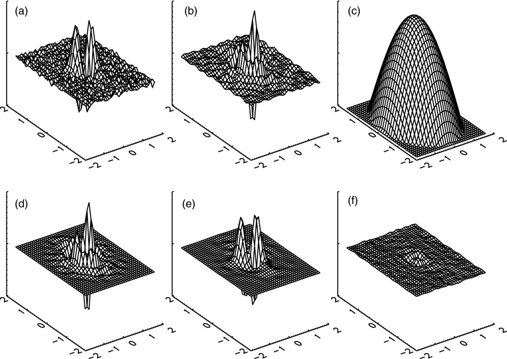