


ABSTRACT
Measurements of polarized radiation often reveal specific physical properties of emission sources, such as the strengths and orientations of magnetic fields offered by synchrotron radiation and Zeeman line emission, and the electron density distribution caused by free–free emission. Polarization-capable, millimeter/sub-millimeter telescopes are normally equipped with either septum polarizers or ortho-mode transducers (OMT) to detect polarized radiation. Though the septum polarizer is limited to a significantly narrower bandwidth than the OMT, it possesses advantageous features unparalleled by the OMT when it comes to determining astronomical polarization measurements. We design an extremely wide-band circular waveguide septum polarizer, covering 42% bandwidth, from 77 GHz to 118 GHz, without any undesired resonance, challenging the conventional bandwidth limit. Stokes parameters, constructed from the measured data between 77 GHz and 115 GHz, show that the leakage from I to Q and U is below ±2%, and the Q − U mutual leakage is below ±1%. Such a performance is comparable to other modern polarizers, but the bandwidth of this polarizer can be at least twice as wide. This extremely wide-band design removes the major weakness of the septum polarizer and opens up a new window for future astronomical polarization measurements.
Export citation and abstract BibTeX RIS
1. INTRODUCTION
Wide-band polarization measurements in millimeter and sub-millimeter astronomy have always been challenging. Examples requiring wide-bandwidth polarimetry measurements include the continuum cosmic microwave background (CMB) polarization observation (Kovac et al. 2002; Kogut et al. 2003; Barkats et al. 2005; Montroy et al. 2006; Sievers et al. 2007; Friedman et al. 2009; Chiang et al. 2010; Bischoff et al. 2011), the synchrotron polarization observations of compact sources (Dowell et al. 1998; Aitken et al. 2000; Culverhouse et al. 2011), the polarization observation of thermal dust emission (Lazarian 2003; Bethell et al. 2007; Hoang et al. 2011), and the observation of Zeeman effects via molecular lines such as CN and SO (Bel & Leroy 1989; Crutcher 1999; Shinnaga & Yamamoto 2000). Except for some particular features of Zeeman effects, most of the above examples focus on linear polarization measurements. For continuum observations, it is desirable for the available frequency bandwidth to be as wide as possible so that the signal-to-noise ratio (S/N) can increase and the spectral index may be determined. For line observations, the emission line can be red-shifted to any unknown frequency when emitted from or absorbed at a distant universe. Hence, wide frequency coverage has a unique advantage.
Though the current trend in CMB polarization experiments has shifted to multi-pixel, silicon wafer-based, incoherent detectors, such as the microwave kinetic inductance detector (Day et al. 2003; Maloney et al. 2010), the conventional, coherent detector still has merit, through its ability to control, detect, and calibrate systematics. In this regard, heterodyne polarimeters with wide bandwidths are highly desirable. For synchrotron emitting compact sources, the interferometry array remains the means of reaching high sensitivity, and it must have coherent detectors for polarization measurements. Similar considerations apply to line and dust emissions from compact molecular cloud cores. All of these factors make the conventional waveguide polarimeter device a time-honored instrument that will always be needed in future forefront millimeter/sub-millimeter telescopes.
Polarization measurements require separating the incoming radiation into two orthogonal components to determine the Stokes parameters. Traditionally two devices have been available for the separation of polarization: the septum polarizer and the ortho-mode transducer (OMT). An ideal septum polarizer can convert an input linear polarization wave into two circular polarization waves of equal power at two output ports. Interestingly, in a specific arrangement, when the electric field of the input wave is perpendicular to or parallel to the symmetric axis of the septum polarizer, the two output electric fields will be either in-phase or 180° out-of-phase, with the latter being delayed relative to the former by 90° over a finite frequency interval. It then follows that when the input is a circularly polarized wave, it will exit entirely through one output port and the other port has a null output. This novel feature of the septum polarizer makes it distinct from the other simpler device, OMT, which separates an input linearly polarized wave into two components of the electric field parallel and perpendicular to the device symmetry axis at two output ports (Wollock et al. 2002; Mennella et al. 2003). The septum polarizer has been known to perform well only within a relatively narrow frequency range, limited by the appearance of resonances. The OMT, on the other hand, has the advantage of being able to cover a wide bandwidth and has been installed in modern telescopes such as the Atacama Large Millimeter/sub-millimeter Array.
A further comparison of these devices reveals that the septum polarizer is good for measuring Stokes Q(≡ [〈ExEx*〉 − 〈EyEy*〉]/2) and Stokes U(≡ [〈ExEy*〉 + 〈EyEx*〉]/2), or the linear polarization, and the OMT is good for measuring Stokes U and Stokes V(≡ i[〈ExEy*〉 − 〈EyEx*〉]/2), or the circular polarization, where 〈...〉 is the time average. The reasons are as follows. If we consider linearly polarized signals and denote the outputs of the septum polarizer to be the right-hand polarization electric field,  and the left-hand polarization electric field
  , by cross-correlating ER and EL, we obtain Stokes Q as 〈EREL* + EREL*〉 and Stokes U as 〈EREL* − EREL*〉. In practice, one normally needs to amplify the weak incoming signals with gains GR and GL immediately following the polarizer. The constructed Stokes parameters are in effect 〈GRGL〉Q and 〈GRGL〉U, assuming the gains are real (see Section 6 for a discussion of complex gains). If one has an approximate knowledge of the average gains GR and GL, the Stokes Q and U can be determined accurately. This can be achieved with a septum polarizer that measures ER and EL directly. If one adopts the OMT, the Stokes U becomes 〈GxGy〉[〈ExEy*〉 + 〈EyEx*〉] and the Stokes Q becomes
  . While Stokes U can be recovered in a manner similar to how it is determined with a septum polarizer, the recovery of Stokes Q has a serious problem (Bischoff et al. 2013).
This is because the polarized signal is already mixed with the much stronger, unpolarized sky, and the amplifiers introduce substantial, unpolarized noise to the signal. Hence, |Ex|2 and |Ey|2 almost contain the unpolarized radiation, and the recovery of weak polarized signals is reminiscent of the determination of a very small number by subtracting one large number from another large number, for which any small error in the two large numbers will render a poorly determined small number. Therefore, the recovery of Stokes Q is only possible if the amplifier gains  and
and  can be calibrated to a high accuracy. However, due to the presence of gain fluctuations in amplifiers, it is often difficult to yield a well-determined Stokes Q with a telescope equipped with an OMT. On the other hand, when the polarized signal only contains Stokes U and V, a similar argument applies except that we must replace Ex by ER, Ey by EL, and the OMT by the septum polarizer. However, there have rarely been pure circular polarization signals in astronomical observations; hence, the OMT is not normally favored for astronomical polarization measurements and is used mostly for the measurement of Stokes I. (Nevertheless, a sophisticated solution for polarization measurements with the OMT has been proposed; Mennella et al. 2003.) In spite of the septum polarizers advantages, it is not widely used in modern telescopes simply because the polarizer has long been regarded as a narrow-band device. Therefore, it will be a great leap forward in polarimeter instrumentation if this major weakness can be removed. In this paper, we report our work specifically to address this issue.
This paper is organized as follows. We introduce prior works on the septum polarizer in Section 2 and highlight the novel approach of the present work. Section 3 outlines our design principles. In Section 4, we report the measurement results of a polarizer fabricated for our test. We convert the measurement results to the mutual leakage of Stokes parameters in Section 5. The leading-order calibration for reducing the Stokes I leakage to other Stokes parameters is described in Section 6. The conclusion is given in Section 7.
2. SEPTUM POLARIZER
The schematics of a septum polarizer is shown in Figure 1, where a stepped metal septum cuts through a circular waveguide at the midplane, dividing it into two half-circular output ports. For an input Ey, the electric field must rotate 90° to reach the output ports, and the two electric fields at the two output ports are 180° out of phase (Figure 2(a)). By contrast, the input Ex remains intact in orientation and the two output electric fields are of the same phase (Figure 2(b)). The stepped septum serves as an impedance transformer for the input Ey, slowing the phase velocity to create a delay relative to the input Ex. To preserve the input and output powers when both components of the input electric field are present, it follows that the relative phase delay between the two components at the output ports must be ±90°.

Figure 1. Typical configuration of the stepped septum polarizer in a circular waveguide. The vertical component (Ey) and horizontal component (Ex) of the electric field fed into the common port are separated by the septum to become the right-hand polarization component output at port R and the left-hand polarization component output at port L.
Download figure:
Standard image High-resolution image
Figure 2. Field distributions of (a) an Ey input and (b) an Ex input. The electric current smoothly circulates in opposite directions on either side of the common wall (septum) for the Ex input as if no septum ever existed, but the current flows in the same direction on either side of the common wall for the Ey input, so that the septum top edge becomes a stagnation point for charge accumulation. Therefore, a virtual TM01 mode, which has primarily the radial electric field, is excited. A good septum is able to re-convert the virtual TM01 mode back to the TE11 mode as it exits to output ports.
Download figure:
Standard image High-resolution imageThough the principle of a septum polarizer has been known for decades, the key is for the septum polarizer to cover as wide a bandwidth as possible. The very first concept of the septum polarizer is given in Regan (1948). The author conceived a simple picture. While Ex propagates into the polarizer unimpeded, Ey, propagating along a sloping septum in a circular waveguide, must have a slower phase velocity with its orientation turning ±90° on either side of the septum. A more illuminating understanding of the spectums functionality came to light some years later when the septum was regarded as a common wall (Chen & Tsandoulas 1973) that had a spatially varying slot with varying cutoff frequencies (Schrank 1982; Behe & Brachat 1991). The in-phase fields fed into the two half-waveguides causing the current to circulate in opposite directions on either side of the common wall, thereby closing the current circuit at the slot with little disturbance. By contrast, the out-of-phase fields cause the current to flow in the same direction on the two sides of the common wall, and the slot interrupts the current, thereby, altering the impedance. In modern stepped septum polarizers, each step in the septum can actually be regarded as an individual slot. If one alters the slot shape, the septum polarizer may be made equivalent to a single-ridge waveguide. The ridge waveguide has been extensively studied for bandwidth enhancement and for better impedance match (Montgomery 1971; Patzelt & Arndt 1982; Vahldieck et al. 1983; Tucholke et al. 1986; Bornmann & Arndt 1987, 1990; Bornmann et al. 1999). The phase velocity of input Ey is slower than input Ex. This is due to the ridge effect, which lowers the cutoff frequency. A ridge with a spatially varying height yields varying cutoff frequencies and controls various degrees of delay over some frequency interval. A careful septum design can often yield a 90° delay in Ey relative to Ex over some finite frequency interval.
Early developments of the septum polarizer were for phase array applications (Parris 1966). A five-element phase array with receivers installed with sloping septum polarizers was soon reported in a conference where the polarizer achieved 15% bandwidth (Davis et al. 1967). Several years later, the first paper was published in which a stepped septum in a square waveguide was used; the authors reported that the polarizer could achieve an even wider (20%) bandwidth (Chen & Tsandoulas 1973). In the same paper, the authors claimed that the 20% bandwidth was close to the bandwidth limit. After this initial publication, square waveguide polarizers remained popular until 1991 when the first circular waveguide polarizer with a stepped septum was made (Behe & Brachat 1991). Circular waveguide polarizers have the advantage that the interface to the front-end feed horn is natural without the need of a transformer, and they have since been widely used in antenna arrays (Kumar et al. 2009; Franco 2011; Galuscak et al. 2012).
Early investigations of the septum polarizer were limited to methods of trial-and-error. The first analysis of a slot septum was conducted based on the Wiener–Hopf method (Albertsen et al. 1983). Subsequently, the mode-matching method, generalized transverse resonance method, and finite-element method were suggested as design improvements (Ege & McAndrew 1985; Behe & Brachat 1991; Esteban & Rebollar 1992). In these studies, the excitations of high-order TE and TM modes presented major challenges, thus making it necessary to adopt the single-value decomposition method of isolating the excitation modes from the fundamental mode (Labay & Bornmann 1992). It was not until 1995 that an optimized square waveguide, four-step septum polarizer was reported (Bornmann & Labay 1995). That work provided detailed analyses of the dimensions of the steps and the thickness of the septum. Like (Chen & Tsandoulas 1973), these authors also claimed that the polarizers maximum bandwidth was about 20%.
We sum up this brief review by listing three key issues often discussed in the literature concerning septum polarizers. First, the bandwidth of the septum polarizer is primarily limited by that of the square (circular) waveguide. Chen & Tsandoulas (1973) suggested that a square (circular) waveguide has a ratio of 1:1.4 (1:1.3) for the cutoff frequencies of the TE01 (TE11) mode and the TE11 (TM01) mode, therefore, the maximum bandwidth of the fundamental mode is at most 34% (26%). If the intervals of the lowest 12% and the highest 2% bandwidths, where the polarizer performance is difficult to control, are avoided, one is left with only 20% (12%) bandwidth for use. Even with further refinements in the septum design, one can achieve at most 25% (15%) bandwidth. Exceeding this limit is the excitation of high-order modes, which can alter the phases of the fundamental modes and produce resonances. An increase in the step number will not help, as the bandwidth limit considered above has been so fundamental that it cannot be broken (Bornmann & Labay 1995).
Second, impedance mismatch between the septum polarizer and the connecting waveguides can also be an issue. There is a tendency for the septum polarizer to lower the pass band, hence to compensate for this, the polarizer must be made smaller by as much as 25% of its normal size. Thus, this creates an impedance mismatch problem for the polarizer's interfaces to other typical waveguides, an issue that was noted in earlier studies (Parris 1966).
Third, the 90° phase shift of Ey, relative to Ex over a wide bandwidth, may be achieved by either the placement of an auxiliary Teflon thin plate next to the metal septum (Chen & Tsandoulas 1973), or the adoption of corrugated walls in the waveguide (Ihmels et al. 1993). The corrugated wall has long been regarded as a phase shifter (Simmons 1955). However, these improvements are impractical in high-frequency applications. Typical dimensions of the polarizer are too small for precision arrangements of extra components or for fabrication of a complicated waveguide interior.
In this work, we report a novel design of the septum polarizer that yields good solutions to all of the issues listed above. We find it possible to break the aforementioned bandwidth limit by carefully optimizing the septum steps for suppressing high-order excitations and resonances over an unprecedentedly wide bandwidth. The circular waveguide septum polarizer reported here can reach a 42% bandwidth. Moreover, the dimension of the polarizer input/out ports are only 10% smaller than normal, making it easy to join other waveguide components with unsophisticated impedance transformers. Most importantly, this septum polarizer, without any Teflon plate or corrugated wall for additional fine tuning, has been designed for high-frequency applications, specifically for the W band, and has been fabricated by conventional machining tools. An extension of this 42% bandwidth design to the G band is also envisioned, challenging the 10% bandwidth G-band polarizer that was reported recently (Leal-Serillano et al. 2013).
3. SEPTUM DESIGN
A circular waveguide is adopted for this polarizer. We challenge the conventional notion of the forbidden band of the Ey input, where high-order TM01 modes are to be resonantly excited. In fact, a virtual TM mode is always excited in the polarizer (Figure 2(a)) due to the intrusion of the septum, so that Ey can rotate 90° and be transmitted as Ex at the output. However, the virtual TM mode may become a real TM01 mode and get reflected back to the input port. One of our septum design guidelines is, therefore, to prevent the virtual TM mode from becoming a real TM01 mode. This guideline can be relatively easy to meet below the TM01 excitation frequency. As there is no mode conversion between the input and the reflection, the usual λ/4 rule applies. However, the guideline becomes questionable beyond the TM01 excitation frequency, for which the virtual TM01 mode can become a real TM01 mode upon reflection, a process that involves mode conversion. The difficulty in handling mode conversion has discouraged prior works from attacking the high-frequency regime, thereby drawing a bandwidth limit.
Nonetheless, careful design of the septum can still suppress the real TM01 mode beyond the excitation frequency. While a very low level of the real TM01 mode is unavoidably excited, it is imperative that the reflected real TM01 mode be smoothly transmitted through the input port and radiate away without a second reflection back to the polarizer interior. This consideration leads to what we call the problem of multiple reflections. When the virtual TM mode is excited, it propagates at a slower speed than the original TE11 mode so that the input Ey is delayed relative to the input Ex. To create a delay of exactly 90°, the wave internal reflections along the five-step septum must occur for the adjustment of the tempo. Too many or too few multiple reflections in the virtual TM mode can yield delays different from 90° and forbid the wave from reaching the output ports. In most frequencies, one can tune the septum steps to yield a delay close to 90°. However, at some discrete frequencies, the septum tuning may fail and the virtual TM modes get severely multiply reflected (or trapped) within the polarizer where they become real cavity modes, which produce resonances. Hence, complete elimination of these cavity modes, especially the one near the TM01 excitation frequency, is the main challenge for an extremely wide-band polarizer.
Our primary design principle for the septum is, therefore, to strictly prohibit cavity modes from occurring at the expense of allowing for some low level of real TM01 excitations, which are to be radiated away through the input end. We begin with a size free design; when the widest percentage bandwidth is identified, we then fix the device size in accordance with the range of frequency desired. In the present case, the range is 80–116 GHz. Given the circular waveguide, we optimize the five-step septum with the height and the width of each step as optimization parameters. The optimization procedure begins with the λ/4 rule for modes of different frequencies. To be specific, the lowest step aims to minimize the reflection of the 110 GHz fundamental, the second and third steps combine to minimize the reflection of the 85 GHz fundamental and the excitation of the 110 GHz high-order mode, and the fourth step aims to control the 95 GHz high-order excitation and the highest step for overall performance tuning. The above setup is used as the initial configuration for the search of optimal parameters.
An Ansoft HFSS 13.0 (High Frequency Structure Simulator) was used to compute the scattering (S) parameters that serve as optimization indicators. The left–right symmetry of the polarizer allows us to compute only half of the space so as to speed up the parameter search. After the optimal parameters are found, we employ the full space simulation to re-compute S parameters as a confirmation check, and to determine the precision tolerances of fabrication. Note that if high-order modes were not allowed to be present as input/output eigen-modes in the HFSS simulation, these high-order excitations would not be able to transmit away from the polarizer. This would produce a large number of multiple reflections and the results would always yield erroneous strong resonances.
We indeed find an optimal solution free of resonance, not only across the entire W-band but also extending beyond 120 GHz. The optimized polarizer aperture is found to be 2.5 mm with the TM01 excitation frequency at 93 GHz. The optimized septum width is found to be 8% of the polarizer aperture, 0.2 mm, for good performance at high frequency and for the mechanical rigidity of a bronze septum. The optimized HFSS results are shown in Figure 3, where the TE11 modes (Ex, Ey) at the common port are denoted as mode 1, the TE11 mode at R/L ports as mode 2, the excited TM01 mode as mode 3, and the excited TE21 mode as mode 4. Here, the S parameter is defined as:
It is found in Figure 3 that the input reflections S11(Ex) and S11(Ey) are under −20 dB and S31(Ey) under −14 dB within 94–118 GHz. The high-order mode TM01 cannot be excited by the Ex input, and S31(Ex) is indeed close to zero. The transmission S21(Ex) is nearly perfect; however, S21(Ey) has some loss due to energy conversion to the high-order mode beyond 93 GHz, and the loss is at most 0.2 dB between 94 and 100 GHz and 0.3 dB at 118 GHz. We find that the excitation of the TM01 mode is unavoidable beyond its cutoff frequency, and beyond 118 GHz an even higher-order mode, TE21, begins to be significantly excited for both Ey and Ex inputs. Nevertheless one can manage to keep the high-order excitation level low up to at least 118 GHz. In particular, the simulation results in Figure 3 show that avoidance of resonances can be achieved over a very wide frequency range (75 to >120 GHz), thus opening a new regime of operation for a waveguide septum polarizer.
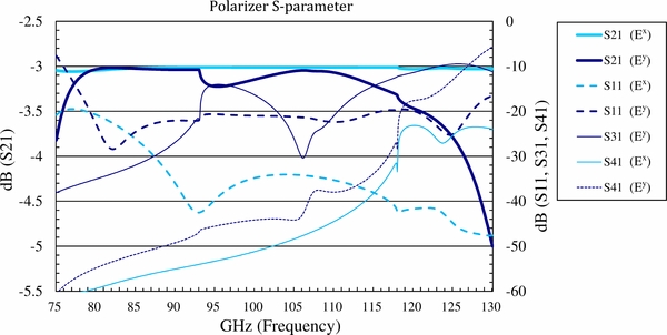
Figure 3. Simulation results of the transmission S21 and the reflection S11 of the fundamental TE11 mode, and of the reflected TM01 (S31) and TE21 (S41) modes, for our optimized septum polarizer. These simulation results are for an ideal polarizer, where left–right symmetry is obeyed. For the Ey input, the TM01 is seen to be well suppressed except near the TM01 cutoff frequency, 93 GHz. Even near this frequency the suppression is still good at the −14 dB level with an insertion loss of 0.2 dB. Most impressively, this polarizer design has been tuned to eliminate all resonances across the entire W-band and beyond 120 GHz. The higher-order mode TE21 begins to be excited beyond 118 GHz for both Ey and Ex inputs, and the transmission S21 for the Ey input deteriorates rapidly beyond 120 GHz.
Download figure:
Standard image High-resolution imageTo provide evidence that the septum design is close to the optimum, we change the waveguide diameter by ±8%, leaving the septum shape and dimension intact. Figure 4 depicts the HFSS simulation results of these changes for the Ey inputs, which are more sensitive to optimization parameters than the Ex inputs. The obvious differences are the shifted frequencies that scale inversely with the diameter. We rescale the frequency axis of S21 in Figure 3 by ±8% and plot S21's in Figures 4(a) and (b), which provide a detailed comparison between the altered configurations and the optimal configuration. The change in diameter causes a slight decline in performance, demonstrating that the polarizers present design is very close to the optimum.
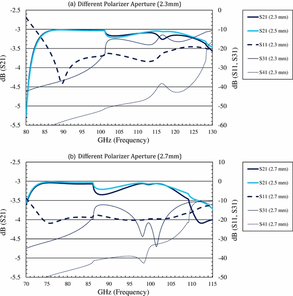
Figure 4. Simulation results of circular polarizers with (a) 8% smaller and (b) 8% larger diameters. To test performance optimization, the septa in these polarizers are the same as that found in the original polarizer which measures 2.5 mm in diameter. The S21 of Figure 3 is rescaled in frequency and over-plotted in (a) and (b) for detailed comparisons. The performance of both polarizers is found to be slightly worse than the original one.
Download figure:
Standard image High-resolution image4. MEASUREMENTS
Before proceeding to the presentation of measurement results, we find it important to stress the arrangements before the signal enters the polarizer from the common port. This polarizer operates in the frequency range beyond the cutoff of TM01 excitation. Despite our ability to suppress the high-order excitation to a great degree, there is still some low level of TM01 mode that gets reflected back to the front-end devices. If the front-end devices do not allow the TM01 mode to radiate, the reflection of it from the front-end back to the polarizer interior will lead to a cavity effect and create spurious new resonances. It is therefore essential that the front-end device permit total transmission of TM01 modes. The condition is naturally fulfilled in the telescope setting since the polarizer is preceded by a feed horn, which allows the reflected TM01 mode to radiate away. However, the radiation boundary condition cannot be satisfied when we perform measurements by connecting the common port of the polarizer to the rectangular waveguide of the measurement device. In this case, the excitation mode is totally reflected back to the polarizer, thereby producing new resonances.
The polarizer is measured by the HP 8510 vector network analyzer (VNA) which covers 75–115 GHz. Two types of measurements are made. For measurement A, the common port is the output port of the polarizer, which is connected to a Potter feed horn (Leech et al. 2012), and the R and L ports are connected to the two ports of VNA. For measurement B, one port of VNA is connected to the common port via a rectangular-to-circular waveguide transition adapter and the other port of VNA to the R (L) port, with the L (R) port properly terminated. Measurement A tests the performance of the R/L ports return loss and mutual isolation. If a high-order mode is excited away, then there can be no telling of the high-order excitation in measurement A. However, if there are internal multiple reflections, i.e., cavity modes, inside the polarizer, measurement A can reveal resonances. On the other hand, measurement B must use a transition adapter between the VNA and the common port, which can cause a serious problem in reflecting the excited TM01 mode back to the polarizer, creating the otherwise absent resonances in the VNA measurement. Nevertheless, if one ignores the responses at some discrete resonances and reads only the continuum results, measurement B can provide the full characteristics, and thus the full Stokes parameters, of the receiver polarizer.
- 1.Measurement A. Figure 5 summarizes the results. First of all, no resonance appears in this measurement. In the interval between 85 GHz and 115 GHz, the return loss and the isolation are largely below −20 dB. The slight rise of return loss to −17 dB in the low-frequency interval 77–85 GHz is due to the slight mismatch between the WR10 rectangular waveguide of the VNA and the polarizer semi-circular waveguide. We verify the measurement results by simulating the exact measurement configuration with HFSS, finding good agreements, especially in low frequency, where the waveguide mismatch prevails. This is a minor problem that can be easily corrected by a transition adapter.In the past, the polarizer was found to show resonances above the excitation frequency of high-order modes in measurement A, from which the bandwidth limit mentioned in Section 2 was set. For the detection of resonances, A is a reasonable measurement because when multiple reflections of high-order modes in a cavity occur, part of the high-order modes should be converted to the fundamental mode back to the input and isolation ports. This can thus reveal the presence of resonances, though the conversion efficiency may be low. We find no resonance to be present in measurement A, providing evidence against the presence of a cavity mode inside the septum polarizer. Full justification of this claim requires the input to be injected from the common port, and it leads us to measurement B.
- 2.Measurement B. As mentioned earlier, measurement B cannot be free of problems since the VNA rectangular waveguide port produces multiple reflections of TM01 modes in the polarizer. Hence, spurious resonances are always present in this measurement. To circumvent this difficulty, our solution is to change the length of the rectangular-to-circular transition waveguide and examine whether any identical resonance exists regardless of such a change. The rationale behind this approach is that if any internal cavity mode is to exist, its resonance frequency should be independent of the length changes of the external reflector. Our measured results will be further checked against the HFSS simulations to ensure the correctness of the interpretation.

Figure 5. Results of isolation Sij and reflection Sii for measurement A, and results of the simulation with an identical setup as the measurement. The overall agreement between the two is very good. The measured S12 turns out to be indistinguishable from the measured S21.
Download figure:
Standard image High-resolution imageFigure 6 presents results for the Ex input and for the Ey input, respectively. Here the length of the circular waveguide section in the transition adapter is chosen to be the shortest possible, 0.2 mm. The result for the Ey input reveals three resonances at 95.2 GHz, 104.2 GHz, and 110.2 GHz, and the HFSS simulation yields exactly the same resonances. The result for Ex reveals an unexpected single resonance at 95 GHz. This odd resonance is actually produced from the mutual leakage between Ex and Ey, due to axis misalignment by 1 8 at the interface between the rectangular-to-circular transition adapter and the polarizer. The misalignment has also been verified by the HFSS simulation, shown in Figure 6 as well. We note in Figure 6 that the power imbalance of R and L ports in input Ex and input Ey measurements tends to be opposite. This result is also caused by the 18 axis misalignment, a problem that can be further verified by the mutual leakage of Stokes Q and U discussed in the next section.
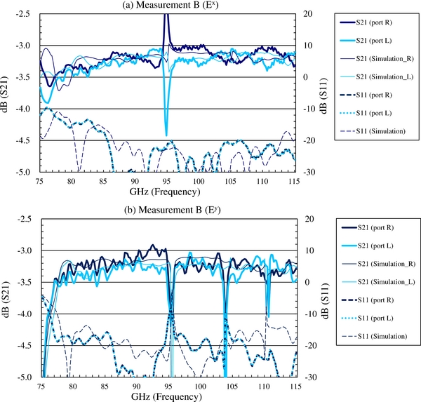
Figure 6. (a) Measurement B and simulation results for the Ex input and (b) the Ey input. The rectangular-to-circular transition adapter is 0.2 mm in length. The unexpected resonance at 95 GHz shown in (a) is due to slight axis misalignment of 18 at the interface between the adapter and the polarizer. The agreement between measurement and simulation is considerably good, especially the measured resonances, are all captured by simulations. Again, we find the measured S11's for both R and L outputs are almost identical.
Download figure:
Standard image High-resolution imageOther than these discrete resonances, the polarizer performs well in the continuum, with about 0.2–0.3 dB additional power loss compared to the ideal polarizer simulation results. This additional loss is partly caused by the transition adapter before and a splitter after the polarizer. The output power imbalance between R and L ports in the continuum is also small, within 0.2 dB on average and 0.3 dB maximum, despite the fact that half of the power imbalance is produced by irrelevant axis misalignment. (In real telescope applications, the rectangular-to-circular transition adapter will not be present, and the axis misalignment will not be an issue of concern.) The phase at every frequency has also been measured, but is not shown here. These phase measurements are important for our further examination of the mutual leakage among four Stokes parameters in the next section.
Figure 7 basically presents the same measurements as Figure 6, but with different sets of rectangular-to-circular transition adaptors of 5 mm and 10 mm in length. The resonances in this case are more closely packed than the previous case, somewhat deteriorating the performance in the continuum. Hence, we shall focus on the identification of resonances per se. The resonances in the measurements are located at 92.4 GHz, 95.6 GHz, 101.2 GHz, 105.4 GHz, and 109.6 GHz for the 5 mm adaptor and 92.0 GHz, 93.4 GHz, 95.8 GHz, 99.4 GHz, 103.4 GHz, 106.0 GHz, 109.6 GHz, and 114.2 GHz for the 10 mm adaptor. Together with Figure 6, we find that none of these resonances is in common in all three cases of different external cavity lengths, indicative of no internal cavity mode in the polarizer. We also find that all measured resonances coincide with the simulation resonances. The confirmation of measurements by simulations further reinforces our confidence that this polarizer is free of resonance over the measurement range from 75 GHz to 115 GHz. The faithful reproduction of the measured results by simulations in turn makes it believable that the polarizer design should be free of resonance, even beyond 120 GHz, as indicated by the simulation presented in Figure 3.

Figure 7. Measurement B and simulation results for Ey inputs where the original 0.2 mm adapter is replaced by two other adapters of (a) 5 mm and (b) 10 mm in length. The measured extra losses <0.3 dB compared with simulation results are likely caused by the ohmic loss in the adapters. Nevertheless we find all measured resonances are captured by simulations.
Download figure:
Standard image High-resolution image5. POLARIZATION LEAKAGE
A number of minor imperfections in the polarizer lead to small leaks among different Stokes parameters. In view of the weak polarized signal in the presence of the stronger unpolarized source, the primary concern of a polarizer is the leakage from Stokes I to the other three Stokes parameters. Other less critical concerns include the mutual leakage among the three polarized components. Since the observed polarized radiation is mostly linearly polarized, the Stokes V is zero, and the polarization mutual leakage is between Stokes Q and U. As long as the Q − U leakage is controlled within the few-percent level, the performance of the polarizer is considered to be acceptable (Leitch et al. 2002). However, in very demanding observations, such as the B-mode polarization observations of the CMB radiation, it is the level of Q − U leakage that sets the sensitivity limit of an instrument (Hu et al. 2003; O'Dea et al. 2007). Below, we compute the mutual leakage of the four Stokes parameters from the data of measurement B with the 0.2 mm transition adapter.
The output complex electric fields at the R and L ports for an ideal septum polarizer are expressed as:

for an ideal septum polarizer. Consider different polarizers inside a pair of receivers (m, n). The visibility is known as the time-averaged cross-correlation of the complex electric fields incident to receivers m and n, and the correlation responses are obtained as:
The co-polar (ERER, ELEL) correlations provide information about I and V and the cross-polar (EREL, ELER) correlations about Q and U. For simplicity, we consider a radiometer polarizer as an example with m = n = 1 and drop the receiver indices. We model the imperfect responses of the ER and EL outputs after the amplifiers as

where ΔR, L and εR, L denote the magnitude losses of Ex and Ey at ports R and L, and αΔ, αR, and αL denote the phase errors in reference to Ex at the R port. Here, ΔR, L, εR, L, αΔ, αR and αL are of the same order of smallness O(η). Here, η < 2% from the VNA measurements, and the leading-order corrections suffice to compute the leakage. We also take the amplifier gains, GR and GL, to be real. This is because the relative phase between the two complex gains and the relative path delay in  and
and  can be pre-determined and calibrated out. Hence after the phase calibration, the gain can be made a real quantity. The correlations of the two amplified electric fields now become:
The above four expressions contain the leading order Stokes parameters, Q, U, V, and I, followed by the leakage from the other three Stokes parameters on the order O(η). The leakage obeys a symmetry principle as a result of the scattering matrix being unitary or the quantity I2 − (Q2 + U2 + V2) being an invariant if no loss were to occur. The leakage coefficients between Q and U, Equations (5.4c) and (5.5b), are the same in magnitude but opposite in sign, indicating that the antenna principal axes are not perfectly aligned with the polarizer axes and rotate by a small amount. The coefficients of leakage from I to Q, U and V, Equations (5.4a), (5.5a) and (5.6a), respectively, are the same as those of the leakage from Q, U, and V to I, Equations (5.7b), (5.7c), and (5.7d), when the two gains are the same GR = GL. The leakage between Q and V, and that between U and V, also have the same magnitudes, but opposite signs when GR = GL. Finally, the net loss in Stokes I, Equation (5.7a), is the same as the loss in Q, Equation (5.4b), in U, Equation (5.5c), and in V, Equation (5.6d), again when GR = GL. Hence, without amplifiers, the leakage in a septum polarizer is determined by six parameters, three from the amplitude imbalance, i.e., ΔR + ΔL −  R − L, ΔR − ΔL + R − L, and ΔR − ΔL − R + L, and three from the phase imbalance, i.e.,
  ,
,  , and
, and  . If the polarizer is lossy, there will be an additional parameter, ΔR + ΔL + R + L, that gives uniform suppression of all four Stokes parameters.
Taking the VNA measurement data for two individual septum polarizers fabricated with the same design, we can compute various leakage coefficients according to the formula given above. As the measurements involve only VNA with no amplifiers, we let GR = GL = 1. In Figures 8 and 9, we plot the leakage from I to other three polarization components and the polarization mutual leakage. The measurement results are consistent for the two polarizers, and they are summarized in Table 1. Clearly the leakage is systematically different below and above the excitation frequency at 95 GHz, despite the fact that they are both small. Given the finite line widths of the three resonances presented in Figure 6, the measured results of the nearby continuum are likely contaminated by the poor responses at the resonances. Therefore, the leakage should be regarded as pessimistic, and the actual performance should be better than the results indicated here. We additionally find that the mechanical requirement of the polarizer has no major bottleneck, judging from the performance consistency of the two polarizers.

Figure 8. Measured leakage from Stokes I to polarized components, ( ,
, ,
,  ) for the two modules (a) and (b). The partial differentiations are taken on Equations (5.4)–(5.6).
Download figure:
Standard image High-resolution image
Figure 9. Measured leakage among the polarized components Q, U, and V for the two modules (a) and (b). The Q − U mutual leakage has a major contribution from the axis misalignment of the measurement adapter, and the resulting phase error has been corrected in this figure. Note that the V − U leakage is a few times larger than the others.
Download figure:
Standard image High-resolution image
Table 1. Summary of Polarization Leakage
| Leakage | 77–95 GHz | 95–115 GHz |
|---|---|---|
| I to Q | 1% to − 1% | 2% to 0% |
| I to U | 0% to − 1% | 1% to − 2% |
| I to V | 1.5%–0.5% | 1%–0% |
| Q to U | 0.5%–0% | 0% to − 0.5% |
| Q to V | 0% to − 1% | 0% to − 2% |
| U to V | 0% to − 8% | 5% to − 8% |
Download table as: ASCIITypeset image
6. CALIBRATION FOR REMOVING LEAKAGE FROM STOKES I
Given the estimated leakage of this polarizer, from the large Stokes I to other three small Stokes components, one can perform further calibrations at the system level to further reduce the I leakage of the 2% level. To the leading order, only the leakage from the much stronger, unpolarized component to the polarized component is to be calibrated out. Higher-order calibrations are possible, but this subject is quite involved and will not be discussed here. Again, we take the simple case of a radiometer, where the single receiver outputs, GRER and GLEL, are to be correlated to obtain the four Stokes parameters. In contrast to Sections 1 and 5, here GR and GL are now taken to be complex, including system phase delays. With an unpolarized source as an input to a perfect receiver, one would obtain a finite value for Stokes I and zero values for other Stokes components. Non-zero values in other Stokes components in a real system represent the instrument leakage that is to be removed. The first part of system calibration can be conducted in the laboratory and determine the coefficients presented in Equations (5.4)–(5.6) from the four non-zero Stokes parameters. The second part of the calibration is to be conducted in the field so that the Stokes I leakage can be subtracted away from the observed, polarized components.
The magnitudes of the gains GR and GL can be determined from the power measurements of the two outputs, |GRER|2 and |GLEL|2, with the receiver exposed to an unpolarized source of known temperature. Determination of the relative phase between GR and GL is tricky, requiring a variable delay to alter the relative phase between GRER and GLEL. For a finite bandwidth source, the delay cross correlation between GRER and GLEL will create fringes with an amplitude modulation as a function of the delay. The zero delay between GR and GL is one for which both amplitude modulation and fringe are the maximum. When calibration is to be performed with frequency resolution, digitization of data is required for the determination of complex gains per frequency, GR(ν) and GL(ν). All the above tasks can be conducted in a well-controlled laboratory and hence the complex gain GR and GL can be measured at high precision.
Once the complex gains are determined, the leading order leakage of Stokes I to other three Stokes components, Equations (5.4a), (5.5a), and (5.6a), can then be measured with an unpolarized source. Unlike the VNA measurement results presented in Section 5, which are affected by spurious resonances, the quantities (ΔR + ΔL) − (R + L),  , and (ΔR + R) − (ΔL + L) can be directly determined at the system level.
In the field, where other three Stokes parameters are much smaller than Stokes I by a factor of O(δ), with δ ≪ 1, it is necessary to measure Stokes I in order to construct the I leakage according to Equations (5.4a), (5.5a), and (5.6a). However, the removal of I leakage to Stokes V may be difficult to perform in the field due to the gain fluctuations, and therefore, a poorly determined Stokes V is expected. After the calibration, the leakage from Stokes I to Stokes Q and U can theoretically be removed up to O(η2) compared to the polarized components, since I can in turn be contaminated by leakage from Q, U, and V (cf. Equation (5.7)). In practice, the accuracy of the measured Stokes I places a limit on the degree of removal of the I leakage.
For example, assume that the gains can ideally be determined accurately after a long integration, and the weak linear polarization signals are detected with S/N = 10. The Stokes I must have already been measured with a high S/N of about O(10δ−1). With a measurement error of order δ/10 in Stokes I, the leakage from the unpolarized component to polarized components can be removed up to O(η/10) of the polarized components. Although the residual is not as small as O(η2), it is still much smaller than the polarization mutual leakage O(η). On the other hand, the mutual leakage among Stokes Q and U cannot be reduced by the leading-order calibration since Q and U are weak with a relatively low S/N, unlike the strong I. It is, therefore, up to the performance of the polarizer to limit the leakage, and in our case the Q − U mutual leakage is < ± 1%.
In sum, after the leading-order removal of the Stoke I leakage, the polarized components can be made accurate up to order O(η) contributed primarily by the Q − U mutual leakage. Higher-order calibration is possible with an even deeper integration, provided that the receiver system is sufficiently stable.
7. CONCLUSION
In this paper, we report a novel design of a septum polarizer that has a 42% well-performing bandwidth, from 77 GHz to 118 GHz as opposed to the conventional notion of about 20% maximum bandwidth. The conventionally alleged maximum bandwidth was derived primarily from a consideration of a limit set by the cutoff frequency of the fundamental modes and the excitation frequency of high-order modes. Our polarizer, adopting a circular waveguide, and housing a five-step septum, is able to break the upper bandwidth limit and extends the usable frequency into the range where high-order TM01 modes are excited. This is made possible because we have uncovered an under-explored regime in which TM01 excitations can be severely suppressed and TM01 resonances can be entirely eliminated. Particularly near the TM01 excitation frequency, the septum can manage to avoid multiple reflections of the long wavelength modes inside the polarizer. In addition, the mutual leakage among all four Stokes parameters has been measured. It shows that this septum polarizer performs well, having I to Q, U leakage less than 2%, and Q − U mutual leakage less than ±1% in almost all frequencies.
A few dozen polarizers of our design have been fabricated by conventional precision machining with ±5 μm tolerance, and most of them perform similarly to the two modules reported here. Due to the simplicity of the polarizer without any complicated component to assist widening the bandwidth, it sets a milestone for the instrumentation of polarization measurements.
This septum polarizer will be installed in an upgraded National Taiwan University (NTU)-Array prototype, where each receiver is equipped with 19 pixels of coherent detectors. The 80–116 GHz signals collected by the upgraded NTU-Array are to be processed by digital correlators that are designed to simultaneously cover the 36 GHz bandwidth for all pixels in all receivers with a frequency resolution down to 100 kHz using software correlation. In the context of this work, the backend digital processing capability of the telescope can help calibrate these polarizers with fine frequency resolution.
We thank Dr. D. C. Niu and Dr. C. C. Chiong for their kind assistance with our VNA measurements and ASIAA for granting us access to their HP 8510. Valuable discussions with Dr. K. Y. Lin are also acknowledged. This project is supported in part by the NSC grants 100-2627-E-002-002 and 100-2112-M-002-018.