


ABSTRACT
We present the results of a program to map the Sh2-235 molecular cloud complex in the CO and 13CO J = 2 − 1 transitions using the Heinrich Hertz Submillimeter Telescope. The map resolution is 38'' (FWHM), with an rms noise of 0.12 K brightness temperature, for a velocity resolution of 0.34 km s−1. With the same telescope, we also mapped the CO J = 3 − 2 line at a frequency of 345 GHz, using a 64 beam focal plane array of heterodyne mixers, achieving a typical rms noise of 0.5 K brightness temperature with a velocity resolution of 0.23 km s−1. The three spectral line data cubes are available for download. Much of the cloud appears to be slightly sub-thermally excited in the J = 3 level, except for in the vicinity of the warmest and highest column density areas, which are currently forming stars. Using the CO and 13CO J = 2 − 1 lines, we employ an LTE model to derive the gas column density over the entire mapped region. Examining a 125 pc2 region centered on the most active star formation in the vicinity of Sh2-235, we find that the young stellar object surface density scales as approximately the 1.6-power of the gas column density. The area distribution function of the gas is a steeply declining exponential function of gas column density. Comparison of the morphology of ionized and molecular gas suggests that the cloud is being substantially disrupted by expansion of the H ii regions, which may be triggering current star formation.
Export citation and abstract BibTeX RIS
1. INTRODUCTION
This paper continues a series presenting maps of the emission of carbon monoxide isotopologues from selected galactic molecular clouds. We have made available, in digital format, maps covering degree-scale areas, with full spatial sampling at an angular resolution of ∼40'', a velocity resolution of ∼0.3 km s−1, and a sensitivity of 0.15 K or better rms noise per pixel in one spectral channel. Previous papers reported on the giant molecular clouds (GMCs) associated with H ii regions W51 (Bieging et al. 2010) and W3 (Bieging & Peters 2011); and on the lower-mass clouds in Serpens (Burleigh et al. 2013) and the NGC 1333 region in Perseus (Bieging et al. 2014). In addition, summary results have been given for molecular clouds associated with the H ii regions Sh2-254-258 (Bieging et al. 2009) and M17 (Povich et al. 2009), and for a selection of Bok Globules (Stutz et al. 2009; Lippok et al. 2013).
In our previous papers, we have argued that the lower-level transitions of CO are the best tracers for measuring the full spatial distribution, dynamics, and physical properties of molecular clouds. In brief, CO is abundant, and the transitions with upper state J ⩽ 3 are relatively easily excited even at low temperatures and densities. Most of the millimeter-wavelength transitions are readily observable from the ground, where low noise receivers offer excellent sensitivity in reasonable integration times. Our mapping program has mainly made use of the J = 2 − 1 transition of CO in the two most abundant isotopologues, 12C16O (hereafter simply "CO") and 13C16O (hereafter "13CO"). In this paper, we also present observations of the J = 3 − 2 transition of CO, in large-area maps obtained with a multi-beam focal plane receiver array. The J = 3 level lies at a temperature-equivalent energy of E/k = 33 K, compared with the J = 2 level at 16.5 K. Thus the J = 3 − 2 line is excited at relatively higher temperatures than the J = 2 − 1 line, and thus offers a useful probe of warmer and denser gas associated with regions of current star formation.
The Sh2-235 Molecular Cloud
The subject of this paper is the molecular cloud that lies in the northern part of the Auriga OB1 association toward the galactic anti-center (R.A. (2000) = 05h40m, decl. (2000) = +35°50'; l = 173 5, b = +26). Within or near this cloud are several visible H ii regions, cataloged by Sharpless (1959) as Sh2-231, -232, -233, and -235. (Sh2-234 lies to the south of the H ii region group within the molecular cloud and is not included in this study.) Of these four H ii regions, Sh2-235 is optically the most prominent because of its surface brightness and size, so the associated region is often referred to simply as the Sh2-235 complex. Observations (through 2008) of this "complex," and of the anti-center region in general, are summarized by Reipurth & Yan (2008). They present optical images showing the relationship among the nebulae and massive stars that recently formed there—see their Figures 1 and 5. The most probable distance to the molecular cloud and associated H ii regions is 2.0 ± 0.3 kpc (Montillaud et al. 2015), based on various published distances to the ionizing stars (Evans & Blair 1981; Porras et al. 2000; Ladeyschikov et al. 2015). This distance places the cloud in the middle of the Perseus spiral arm (Reid et al. 2014). We will assume a distance of 2.0 kpc in this paper. At this distance, 1' corresponds to a linear distance of 0.58 pc in the plane of the sky.

Figure 1. Map of rms noise for CO J = 3 − 2. The intensity wedge is in units of main-beam brightness temperature in Kelvin. The mean value of the rms is 0.50 K, with a standard deviation of 0.17 K. Note that the region mapped in the J = 3 − 2 line differs slightly from that mapped in the J = 2 − 1 line.
Download figure:
Standard image High-resolution imageFor molecular cloud studies, the galactic anti-center has the advantage of being relatively clean in kinematic terms, in contrast to the first and fourth galactic quadrants. There are few molecular clouds that are seen along the line of sight yet lying at different distances from the object of interest, so interpretation of the maps is not significantly complicated by overlapping velocity components. The Sh2-235 complex is an excellent example of a GMC6 being substantially disrupted by the formation of massive stars that ionize H ii regions throughout the cloud. Besides direct dissociation and ionization of the molecular gas close to the ionizing stars, the subsequent expansion of the ionized gas has opened large cavities in the remaining molecular gas. In the Sh2-235 cloud complex, we see H ii regions with diameters from ∼30' to <1' (∼17 pc to <0.6 pc), indicating a range of ages and densities. Surrounding these are molecular features that appear to be partial shells or filaments possibly swept up by the expanding ionized gas. Our high spectral resolution allows us to assess the dynamical state of the cloud and to isolate features in three dimensions of six-dimensional position–velocity space. Such analyses will allow us to test whether star formation is being initiated by compression of the molecular gas, a process often referred to as "triggering." For example, Ladeyschikov et al. (2015) have argued, based in part on data from the present study, that a "collect and collapse" process at the compact H ii region Sh2-233 has led to recent star formation on the boundary of the ionized gas.
The Sh2-235 cloud complex has not been well-studied by the Herschel and Spitzer infrared satellites. Only selected areas, mostly concentrating on the bright H ii regions and immediate vicinity, have been observed, in contrast to the extensive set of Herschel and Spitzer data available for the other clouds that we have observed in this series (W51, W3, NGC 1333, Serpens Main). For example, a limited region of about 20' centered on the Sh2-235 H ii region was studied by Dewangan & Anandarao (2011), who cataloged young stellar objects (YSOs) and classified them according to evolutionary state, using Spitzer IRAC images and ground-based JHK band imaging. Chavarria et al. (2014) presented an extensive analysis of essentially the same field in the Spitzer images but with deeper JHK imaging, and thus were able to identify about three times as many YSO candidates as Dewangan & Anandarao (2011). These studies were limited to about 0.15 square degrees centered on Sh2-235. Infrared point-source catalogs with full-sky coverage now make it possible to identify at least the more luminous candidate YSOs within the entire ∼1 square degree region that we have mapped. We use the 2MASS and WISE databases, along with an algorithm by Marton et al. (2016), to find YSO candidates associated with the Sh2-235 molecular cloud. With at least the more massive YSO candidates identified, we can begin to examine the relationship between current star formation activity and the morphology of the CO emission and ionized gas.
2. OBSERVATIONS AND DATA REDUCTION
All of the observations presented here were made with the Heinrich Hertz Submillimeter Telescope7 on Mt. Graham, Arizona, at an elevation of 3200 m. This facility is operated by the Arizona Radio Observatories, a division of the Steward Observatory at the University of Arizona.
2.1. CO and 13CO J = 2 − 1 Lines
Procedures for the J = 2 − 1 line observations were identical to those described in Bieging et al. (2014). The receiver was the dual-polarization ALMA Band 6 prototype sideband-separating mixer system (Lauria et al. 2006). The spectrometer was a filterbank with 128 channels of 0.25 MHz bandwidth and separation (corresponding to a velocity resolution of ∼0.34 km s−1 for the J = 2 − 1 lines), in each of the two polarizations and two mixer sidebands. The CO line at ∼230 GHz is detected in the mixer upper sideband and the 13CO line at ∼220 GHz in the lower sideband. Each line is observed in both horizontal and vertical linear polarizations, providing independent maps of the emission, which are averaged together to reduce the noise by  . Observations were made during 2010 March–2010 April. The field to be mapped was divided into contiguous 10' × 10' "tiles," each of which was observed in the standard On-The-Fly (OTF) scanning mode. The data were calibrated and processed as described in Bieging et al. (2014). The line intensity calibrator was the compact molecular source W3(OH), with main-beam brightness temperatures and integrated line intensities as given in Bieging & Peters (2011). Telescope pointing was checked and corrected as necessary approximately every 2 hr. The typical pointing error was <5''. Since the transitions of CO and 13CO are observed simultaneously through identical telescope optics and separated in the sidebands of the mixer (see Lauria et al. 2006), the registration of the two isotopologue maps is guaranteed to be correct, ensuring the fidelity of CO/13CO line ratio maps, for example. The pointing errors are in any case a small fraction of the diffraction-limited beamsize (FWHM ≈ 32'').
We applied a modest amount of spatial smoothing to the J = 2 − 1 maps, as done in other papers in this series (see, e.g., Burleigh et al. 2013), by convolution of the maps with Gaussian kernels. The purpose of this smoothing was to make both the CO and 13CO maps have the same resolution (since the diffraction-limited beam sizes differ by the ratio of the line frequencies, ∼5%), and to reduce the noise per pixel. The effective resolution after convolution is 38'' (FWHM), or 0.37 pc at the cloud distance, for both isotopologues. All of the J = 2 − 1 data presented here have been smoothed to this resolution.
Both the CO and 13CO J = 2 − 1 lines were observed with 0.25 MHz filters yielding ∼0.34 km s−1 velocity resolution, but since the line rest frequencies differ by ∼5%, the velocity sampling is not the same for the two isotopologues. Therefore, we resampled the maps by third-order interpolation in velocity on identical LSR values at 0.15 km s−1 intervals, i.e., slightly better than Nyquist sampling.
The observed region of the molecular cloud extended over 70' × 50' (R.A. × decl.), or 41 pc × 29 pc at the cloud distance of 2.0 kpc. Our maps cover the bulk of the CO emission, though the bottom row of tiles was not completely filled out where the line emission appeared to be fading out, due to constraints on observing time. We also observed one additional tile above the topmost complete row, to follow an apparent extension of the emission, but did not fill out a full row due to time constraints. The rms noise in each pixel, computed over a velocity range that is free of CO emission, is uniform to about 30% over the map. The average rms is 0.10 K for CO and 0.12 K for 13CO.
2.2. J = 3 − 2 Line
Observations of the J = 3 − 2 line of CO, at a frequency of ∼345 GHz, were made using the same telescope with a new multi-pixel focal plane array of superconducting mixers ("SuperCam") during the period 2014 April 5–10. For a description of the instrument, see Kloosterman et al. (2012). In brief, the receiver consists of a square array of 8 × 8 superconductor-insulator-superconductor mixers, each with a cooled first-stage IF amplifier. The spectrometer was a custom-built digital Fourier transform spectrometer, which provided 900 spectral channels with a frequency spacing of 0.2686 MHz, or velocity resolution of 0.233 km s−1, for each of the 64 mixers in the array.
Each mixer was calibrated with respect to a fiducial mixer near the center of the array by comparison of measured mixer responses on standard sources. The telescope beam efficiency at the fiducial mixer was measured by observations of Mars, which gave a value of 0.70, with an rms scatter of 1% over multiple measurements. Allowing for systematic calibration errors, we adopt a telescope beam efficiency of 0.70 with an estimated uncertainty of 5%. This value is applied to convert the map to main-beam brightness temperature.
The measured telescope beamwidth was 24'' (FWHM), consistent with the expected diffraction limit and mixer feed horn design. The beam pattern does not show any sign of an error beam or extended large sidelobes, consistent with the measured beam efficiency and the primary reflector surface accuracy, where the rms error of the 10 m paraboloidal surface is ∼25 μm.
Mapping of large areas was done by OTF scanning, with the raster pattern chosen to ensure that each independent pixel in the mapped field is sampled by several of the mixers. The area mapped was covered in several sections, where the telescope was scanned over ∼20'-wide sections in R.A., each extending typically 60' in declination. The sections overlapped in most cases, to reduce the noise. The sections were combined onto a single large map grid with 10'' × 10'' pixels. The data were processed in essentially the same manner as the J = 2 − 1 observations. Spectra were weighted by the inverse of the variance of the noise as determined by the rms of the baseline fit. Only those mixers whose scans sampled a given map position within the convolving kernel contributed to the weighted average spectrum in the final gridded map. Consequently, areas near the beginning and end of the telescope scan, and at the top and bottom rows of each map section, were not as well sampled as the inner parts of the OTF raster pattern, and therefore showed significantly higher noise (i.e., the map edges are vignetted). We trimmed the final map to omit the excessively noisy vignetted regions. Also, not all 64 mixers in the array were in operation, and some had excessive noise and thus were omitted from the data processing. These missing mixers produced some systematic variations in the noise level over the final map due to differences in the effective integration time at different pixels.
To mitigate the effects of non-uniformity in the noise, at least on small spatial scales, we have smoothed the images with a Gaussian kernel with a FWHM of 20'', or 2 pixels in diameter, to reduce the noise and improve the uniformity but without sacrificing much angular resolution. The effective resolution of the smoothed maps is 31'' (FWHM) or 0.30 pc. Figure 1 shows a map of the rms noise for the smoothed image, computed over a range of velocities without CO emission. The central part of the mapped area has the lowest noise due to substantial overlap in the OTF mapping sections. Other variations are a result of variable weather conditions during the observations. Horizontal striping is notable in sections that had no overlapping OTF regions, and where mixers omitted due to excessive noise created variations in the uniformity of the total integration at each pixel. It should be emphasized that even though the smoothed map has some pixel-to-pixel variation in the rms noise, the calibration of the spectra is uniform across the map. The spatial structure of the CO J = 3 − 2 emission is correctly represented, even if the noise levels vary somewhat with position.
3. RESULTS
3.1. Global Spectra
Figure 2 shows the spectra of the three observed CO lines, averaged over the entire mapped areas, for CO and 13CO J =2 − 1 (left panel) and CO J = 3 − 2 (right panel). All three lines show a roughly Gaussian central component and a wing of emission on the redshifted side. The J = 2 − 1 13CO line is about five times weaker and has a narrower Gaussian center than the CO line. These differences, largely a consequence of the differences in opacities between CO and 13CO, are typical of the CO and 13CO isotopologues as observed in other molecular clouds. The CO J = 2 − 1 and 3 – 2 lines have nearly the same line shape, though the redshifted wing in the J = 3 − 2 transition is weaker relative to the peak compared to the J = 2 − 1 transition.

Figure 2. Left: spectra of CO (solid) and 13CO (dashed) J = 2 − 1 lines averaged over the whole mapped region. The spectrum for 13CO has been expanded vertically by a factor of 5. Right: spectrum of CO J = 3 − 2 averaged over the mapped region. Vignetted pixels have been masked out.
Download figure:
Standard image High-resolution image3.2. Peak and Integrated Intensity Maps
Since the lines of the most abundant isotopologue, CO, are generally quite optically thick for our observed transitions, the peak observed brightness temperature is a useful indicator of the cloud kinetic temperature, assuming that the lower CO rotational transitions are collisionally excited and near thermal equilibrium. Under typical molecular cloud conditions of density and temperature, these assumptions are likely to be reasonable. In Figure 3, we show a map of the maximum observed brightness temperature for the CO J = 2 − 1 transition. The CO map (left panel) may be considered as an indication of the gas temperature distribution. The abundant CO isotopologue is detected at low column densities such that the line may not be optically thick, but nevertheless indicates the presence of molecular gas. In the right panel of Figure 3, we show the Digital Sky Survey II red image of this region, with selected contours of peak CO J = 2 − 1 brightness temperature overlaid. The optical image is dominated by nebular emission from the H ii regions, as well as bright stars. One prominent feature in the left panel is the large hole centered near R.A. 05h39m30s, decl. 35°56'. Figure 3 (left) shows the maximum CO brightness temperature regardless of velocity, so the lack of emission means that this area is nearly devoid of molecular gas. This gap in the molecular gas coincides with the location of the H ii region Sh2-231. In contrast, the brighter H ii region Sh2-235 is centered close to the brightest CO emission at R.A. 05h41m, decl. 35°50'. The peak CO brightness temperatures near this more compact, presumably younger H ii region are in the range ∼30–45 K, indicating that some significant heating of the molecular cloud is occuring close to the ionized gas.

Figure 3. Left: peak brightness temperature independent of velocity for CO J = 2 − 1. Color wedge is in units of Kelvin, with a square-root stretch to emphasize lower intensity features. Right: Digital Sky Survey II red image with contours of peak CO J = 2 − 1 brightness temperature overlaid. Contours are at 10, 20, 30, and 40 K. The four main H ii regions are labeled.
Download figure:
Standard image High-resolution imageThe peak brightness temperature of the CO J = 3 − 2 map is shown in Figure 4. The features are very similar to the J = 2 − 1 map, and have similar values for peak temperature, consistent with the J = 2 − 1 and 3 − 2 CO lines both being optically thick over the bulk of the molecular cloud.
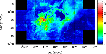
Figure 4. Map of peak beam-smoothed brightness temperature for CO J = 3 − 2 line. Color wedge is in units of Kelvin, with a square-root stretch to emphasize lower intensity features. Note that the region mapped in the J = 3 − 2 line differs from that mapped in the J = 2 − 1 line.
Download figure:
Standard image High-resolution imageBy comparing on a pixel-by-pixel basis the peak intensities of the three observed transitions, we can assess whether the observed CO rotational levels are populated in near-LTE conditions. In the left panel of Figure 5 we plot the peak brightness temperature of the CO J = 3 − 2 versus the J = 2 − 1 lines. The J = 3 − 2 map has been smoothed and re-gridded to match the resolution (38'' FWHM) and spatial sampling of the J = 2 − 1 map. Pixels where the peak intensity is <5 × rms are omitted. The green diagonal lines show the loci of constant brightness temperature ratios. The red curved lines show the loci expected for optically thick emission where the excitation temperatures of the J = 3 − 2 and J = 2 − 1 lines are in the ratios of the red labels, i.e., the red curve for 1.0 corresponds to LTE, the lower curves correspond to sub-thermal excitation, and the higher curves correspond to super-thermal excitation. Here we have calculated the red curves using the definition for the "radiation temperature" in which the observed maps are calibrated, namely

where ![${J}_{\nu }(T)\equiv (h\nu /k)/[\exp (h\nu /{kT})-1]$](https://content.cld.iop.org/journals/0067-0049/226/1/13/revision1/apjsaa3617ieqn2.gif) , τ is the line optical depth at the peak, and we assume the background radiation is only the CMB, so Tbgd = 2.73 K. For the left panel of Figure 5 we assume that both of the CO lines are optically thick so that
, τ is the line optical depth at the peak, and we assume the background radiation is only the CMB, so Tbgd = 2.73 K. For the left panel of Figure 5 we assume that both of the CO lines are optically thick so that  . The majority of points in the graph cluster around the line with Tex(3 − 2)/Tex(2 − 1) = 0.9, suggesting that the CO energy levels are slightly sub-thermally populated for J > 2, but are not far from LTE. A handful of pixels appear to have somewhat super-thermal excitation, which may result from proximity to hot stars, as will be discussed below in Section 3.4.

Figure 5. Left: peak brightness temperature of CO J = 3 − 2 vs. J = 2 − 1 at each mapped pixel. Pixels with peak intensities of less than 5 × rms are omitted. Red curves show loci of constant excitation temperature ratios (labeled); green straight lines show loci of constant observed brightness temperature ratios. Right: peak brightness temperatures at each mapped pixel for 13CO and CO J = 2 − 1. Red lines show loci of constant CO excitation temperature (labeled) for LTE conditions; green lines show loci of constant CO J = 2 − 1 peak optical depth (labeled), also for LTE, assuming isotopic abundance ratio [CO/13CO] = 80.
Download figure:
Standard image High-resolution imageIf the observed CO and 13CO transitions are close to LTE, then the intensities of the J = 2 − 1 isotopologues should indicate both the excitation temperature and the line optical depth. In the right panel of Figure 5, we compare the peak TR values of the J = 2 − 1 CO and 13CO maps for each mapped pixel. (Pixels where the peak intensity is <5 × rms are omitted.) The red curves show the loci of values expected for constant Tex, assumed to be the same for both isotopologues, for a range of CO optical depths from 1 to 100. The green lines are loci of constant CO J = 2 − 1 optical depth, and we assume a CO/13CO abundance ratio of 80 (discussed in Section 3.5 below).
The integrated intensity (or zeroth moment) is another useful quantity to show the distribution of the molecular emission. In Figure 6 we plot the integrated line intensity for the 2 isotoplogues in the J = 2 − 1 transitions. Both maps are integrated over the full range of velocities that show emission, from −28 to −2 km s−1. These maps generally resemble those of the peak line intensity (Figure 4), but with differences that must depend on the width of the lines. For 13CO, the emission is not very optically thick, as will be shown in Section 3.5 below, so the integrated intensity is a fair measure of the total integrated CO molecular column density. If the 13CO abundances were constant throughout the cloud, then the integrated 13CO map would be an indicator of the total gas column density. We also show, as colored crosses and circles in Figure 6, the positions of candidate YSOs that were identified from analyses of the 2MASS and WISE all-sky infrared point-source catalogs (Marton et al. 2016). These objects will be discussed in more detail in Section 3.8.

Figure 6. Maps of brightness temperature integrated over LSR velocity range (−28, −2) km s−1: (left), CO J = 2 − 1 and (right), 13CO J = 2 − 1. The white horizontal lines in the left panel mark the locations of the R.A.-velocity cuts shown in Figure 8. The color wedge is in units of K km s−1, with a square-root stretch to emphasize lower integrated intensity features. Symbols mark the positions of YSOs (see Section 3.8), which are distinguished by evolutionary class: white crosses with black outlines are Class I candidates; magenta open circles are "flat" SED sources; green crosses (with black outlines) are class II; white open circles are class III.
Download figure:
Standard image High-resolution imageA map of intensity for the J = 3 − 2 line of CO, integrated over the same velocity range (−28 to −2 km s−1), is shown in Figure 7 with the same set of symbols marking stellar objects as in Figure 6.

Figure 7. Map of brightness temperature for CO J = 3 − 2 line integrated over LSR velocity range (−28, −2) km s−1. Color wedge is linear, in units of K km s−1. Symbols mark the positions of YSOs (see Section 3.8), which are are distinguished by evolutionary class: white crosses with black outline are Class I candidates; magenta open circles are "flat" SED sources; green crosses (with black outlines) are class II; white open circles are class III.
Download figure:
Standard image High-resolution image3.3. Position–Velocity Maps
Figure 8 shows CO J = 2 − 1 position–velocity maps in R.A. versus LSR velocity, for six cuts at constant declinations (cuts are shown by the horizontal white lines in Figure 6, left panel). This display of the data shows that the dominant CO feature, centered near −20 km s−1 (LSR) extends over nearly the entire range mapped in R.A., with a velocity gradient from more to less negative velocities going from east to west (decreasing R.A.). For example, at decl. = +36° 07', the main CO emission shifts from −24 km s−1 at R.A. = 05h 42m 30s to −17 km s−1 at 05h 37m 30s, implying a velocity gradient of ∼0.2 km s−1 pc−1 in R.A. The structure of the position–velocity maps is more complex than can be described simply by linear gradients, however. Such complexity would be expected for a kinematically disturbed cloud being buffeted by multiple expanding H ii regions. Weaker CO emission is also evident at more restricted ranges of R.A. for velocities nearer to 0 km s−1, which are presumably from smaller molecular clouds nearer to the Sun.

Figure 8. Position–velocity maps of CO J = 2 − 1 beam-smoothed brightness temperature in R.A. vs. velocity at constant declinations, given in the upper left corner of each panel and shown by horizontal white lines in the left panel of Figure 6. Color wedge is in Kelvin, with a logarithmic stretch to emphasize lower-level emission. The vertical axis is LSR velocity.
Download figure:
Standard image High-resolution image3.4. Velocity Channel Maps
A critically important feature of this study is the combination of sensitivity and high spectral resolution, which permits an analysis of the kinematics and dynamical state of the molecular gas. Such an analysis is not possible with observations of the dust thermal continuum, as measured by spacecraft such as Spitzer and Herschel, where the observed emission may originate from a whole range of kinematically distinct dust components with different positions, physical properties, and velocities along a single line of sight.
In Figures 9–11, we show maps of CO and 13CO J = 2 − 1, and CO J = 3 − 2 emission, respectively, in selected LSR velocity channels indicated in the top left corner of each panel. The J = 2 − 1 maps are sampled at 1.35 km s−1 intervals and averaged over 0.45 km s−1. The CO maps (Figure 9) cover a larger velocity range than the 13CO maps (Figure 10) because the CO line has a greater velocity width, but the same sampling of velocity space is presented for both isotopologues. The CO J = 3 − 2 maps (Figure 11) are averaged over 0.7 km s−1, and also spaced by 0.7 km s−1, i.e., the velocity coverage is contiguous. In all three figures, the intensity scale has a square-root stretch to emphasize the lower brightness emission. All of the figures are calibrated in main-beam brightness temperature in Kelvin. The J = 2 − 1 images have an angular resolution of 38'' (FWHM) and a typical rms noise of 0.10 K for the displayed velocity width. The J = 3 − 2 images have a 31'' resolution and an rms noise of 0.31 K for the displayed velocity width of 0.7 km s−1 (averaging over three independent velocity channels).

Download figure:
Standard image High-resolution image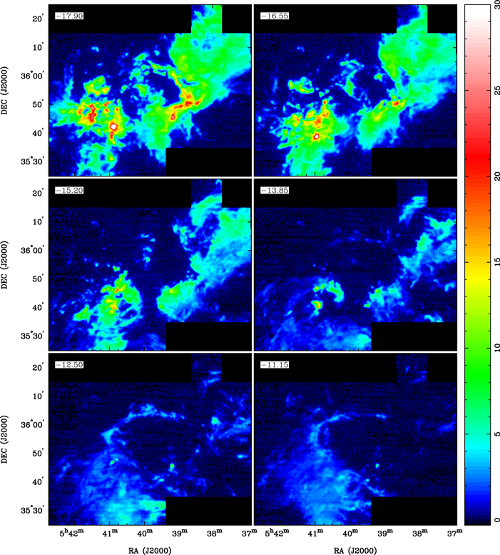
Download figure:
Standard image High-resolution image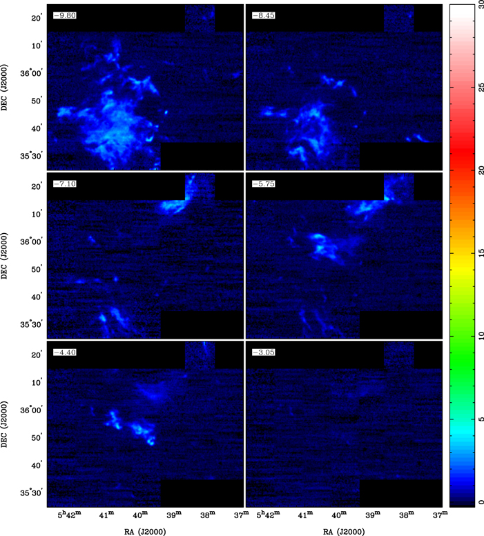
Figure 9. CO J = 2 − 1 spectral channel maps averaged over 0.45 km s−1 and spaced 1.35 km s−1 apart. The mean LSR velocity is in the upper left corners of the panels. Color wedge is labeled in main-beam brightness temperature in Kelvin. The intensity scale uses a square-root stretch to emphasize lower-level emission, with the zero-level offset by −0.3 K (3σ).
Download figure:
Standard image High-resolution image
Download figure:
Standard image High-resolution image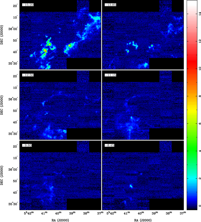
Figure 10. 13CO J = 2 − 1 spectral channel maps averaged over 0.45 km s−1 and spaced 1.35 km s−1 apart. The mean LSR velocity is in the upper left corners of the panels. Color wedge is labeled in main-beam brightness temperature in Kelvin. The intensity scale uses a square-root stretch to emphasize lower-level emission, with the zero-level offset by −0.3 K (3σ).
Download figure:
Standard image High-resolution image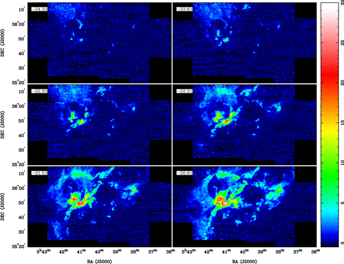
Download figure:
Standard image High-resolution image
Download figure:
Standard image High-resolution image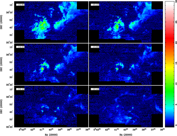
Figure 11. CO J = 3 − 2 spectral channel maps averaged over 0.7 km s−1 and spaced 0.7 km s−1 apart. The mean LSR velocity is in the upper left corners of the panels. Color wedge is labeled in main-beam brightness temperature in Kelvin. The intensity scale uses a square-root stretch to emphasize lower-level emission, with the zero-level offset by −0.3 K.
Download figure:
Standard image High-resolution imageAll of the velocity channel maps show that the molecular gas is in a highly disturbed state, with numerous small-scale clumps and filaments, as well as large holes or gaps between the molecular gas. The most prominent holes are at the positions of the dominant H ii regions, especially at Sh2-231 as noted above, but the other ionized regions also appear to be affecting the associated molecular gas. The structure of the cloud changes significantly with radial velocity, as expected if the gas is in a highly turbulent state, or has organized motions such as expanding shells at the boundaries of the H ii regions. The highest brightness CO is associated with the more luminous stars as shown in Figures 6 and 7.
Besides numerous small-scale features, there are regions of extended diffuse emission at velocities near the line center (e.g., in the range −21 to −15 km s−1) extending over ∼10'–20' (corresponding to 6–12 pc at the cloud distance of 2.0 kpc), where the CO brightness temperature is ∼7–10 K. This diffuse, extended cold gas likely contains most of the cloud mass, as has been shown for other GMCs mapped in lines of CO (e.g., Heyer et al. 1996). The diffuse gas shows up best in the main CO isotopologue, in both the J = 2 − 1 (Figure 9) and J = 3 − 2 (Figure 11) lines. The 13CO J = 2 − 1 line (Figure 10) does not reveal this diffuse cold material as well because of the lower abundance and optical depth of 13CO compared to CO. In contrast to the diffuse emission, all of the compact, bright features are clearly seen in all three of the mapped lines, consistent with high optical depths and excitation temperatures.
If we assume that both the J = 2 − 1 and J = 3 − 2 lines of the main isotopologue (CO) are optically thick and at the same excitation temperature everywhere in the cloud, then the maps should have the same brightness temperatures everywhere. Comparing the line intensity ratios as a function of position and velocity can in principle show areas where one or both of these assumptions fails. In Figure 12, we present ratio maps of the CO J = 3 − 2/J = 2 − 1 brightness temperatures. The J = 3 − 2 map has been convolved to match the resolution of the J = 2 − 1 map (38'' FWHM), and resampled on the same velocity grid. The panels in Figure 12 show velocity channels, averaging over 0.45 km s−1, at representative LSR velocities to illustrate the behavior of the line ratio. Pixels are blanked where the denominator, the J = 2 − 1 line, falls below 0.5 K (5σ). We also show in Figure 12 the locations of (1) the ionizing stars of the 4 H ii regions, (2) compact H ii regions, and (3) some luminous embedded IR sources with associated molecular outflows, all as white crosses with black outlines. The identifications of these objects and their coordinates are given in Table 1. Coordinates are from the SIMBAD database, with ionizing stars as given by Reipurth & Yan (2008), Boley et al. (2009), and Ladeyschikov et al. (2015). The ionizing stars and bright compact IR sources will likely act as heating sources for the associated molecular gas.
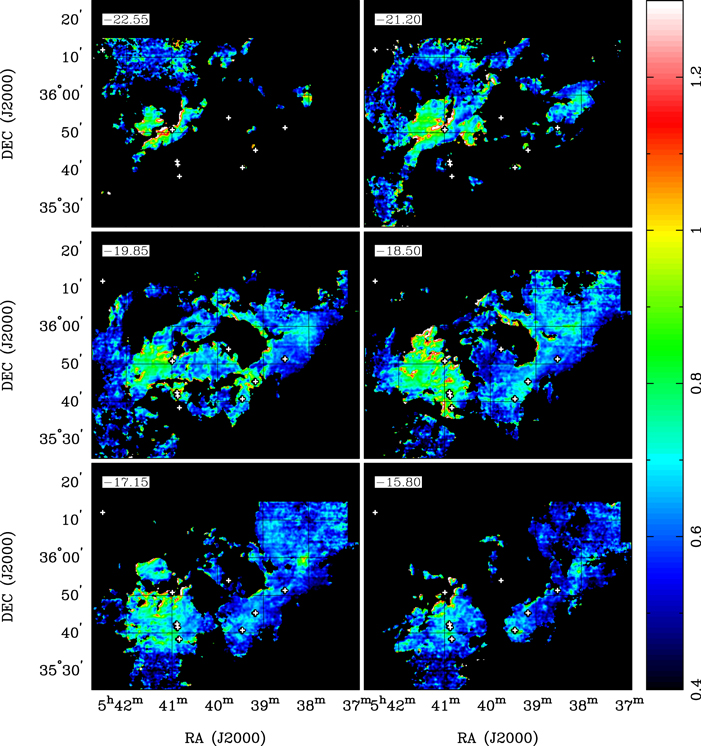
Figure 12. Velocity channel maps of CO (J = 3 − 2)/(J = 2 − 1) intensity ratios. The mean LSR velocity is in the upper left corners of the panels. The white crosses mark ionizing stars, compact H ii regions, or embedded IR sources (see Table 1).
Download figure:
Standard image High-resolution imageTable 1. Ionizing Stars, Compact H ii Regions, and IR Sources in the Sh2-235 Complex
| Identifier | R.A. (J2000) | Decl. (J2000) | Sp. Type | Comment |
|---|---|---|---|---|
| HD 37737 | 05h42m31 16 16 |
36°12'01'' | O9.5IIIa | Ionizing star of Sh2-232 |
| BD+35°1201 | 05 40 59.45 | 35 50 46. | O9.5Vb | Ionizing star of Sh2-235 |
| Sh2-235A | 05 40 53.33 | 35 42 22. | B0.5c | Compact H ii region |
| Sh2-235B | 05 40 52.37 | 35 41 29. | B1Vd | Compact H ii region |
| Sh2-235C | 05 40 50.3 | 35 38 23. | B0.5 | Compact H ii region |
| CGO 103 | 05 39 45.64 | 35 53 56. | O9Vb | Ionizing star of Sh2-231 |
| IRAS 05361+3539 | 05 39 27.7 | 35 40 43. | ... | IR/outflow sourcee |
| IRAS 05358+3543 | 05 39 10.4 | 35 45 19. | ... | IR/outflow sourcef |
| USNO-A2 1200-03588518 | 05 38 31.5 | 35 51 19. | B0.5Vg | Ionizing star of Sh2-233 |
Notes.
abinary. bGeorgelin et al. (1973). cThompson et al. (1983). dBoley et al. (2009). eShepherd & Watson (2002). fBeuther et al. (2002, 2007). gLadeyschikov et al. (2015).Download table as: ASCIITypeset image
3.5. Velocity Moment Maps
The velocity moments of the spectrum can be useful for characterizing the gross properties of the emission, without assuming a specific line shape (e.g., Gaussian). The first moment (centroid) is a measure of the intensity-weighted mean velocity of the emitting gas. In Figure 13, we show the distribution of centroid velocities for the CO and 13CO J = 2 − 1 emission. The moment integral was calculated over the LSR velocity range (−28, −2) km s−1. Pixels where the maximum line intensity within that velocity range was less than 0.5 K (5 × rms noise) are blanked. Most of the CO map (left panel) has a mean velocity of ∼−17 km s−1, but a large area in the northeast of the map has a mean some 5 km s−1 more negative, while a region to the south of Sh2-235 is redshifted relative to the bulk of the cloud, with a mean velocity of about −13 km s−1. There are smaller regions with mean velocities discrepant from the cloud average, by ∼4–5 km s−1.

Figure 13. Maps of centroid velocities (1st moment of the spectrum): (left), CO J = 2 − 1 and (right), 13CO J = 2 − 1. Color wedge is in units of km s−1 (LSR). The moment is integrated over the velocity range −28 to −2 km s−1 for both CO and 13CO. Pixels are blanked if the maximum line intensity is less than 0.5 K ( ) in all channels.
Download figure:
Standard image High-resolution imageThe CO J = 2 − 1 line is generally very optically thick, however, so the velocity centroid is not necessarily a good measure of the true bulk motion of the gas along a line of sight. The 13CO J = 2 − 1 line should be a better measure of the gas motions. In the right panel of Figure 13 we show the 13CO velocity centroid, also integrated over the same range of LSR velocities as the CO map. The 13CO centroid distribution shows more small-scale structure, perhaps consistent with the disturbed morphology of the velocity channel maps, and with turbulent motions resulting from the expansion of H ii regions. Gradients on the order of 5 km s−1 over distances of ∼1'–2' (0.6–1.2 pc) are evident at several locations, especially near the dominant H ii region Sh2-235.
The second velocity moment, or dispersion (σV), gives a measure of the line width at each pixel. In Figure 14, we show maps of the CO and 13CO J = 2 − 1 velocity dispersions, where the moment integrals are computed over the same velocity range as for the first moment, and pixels with peak intensity ⩽5× rms are blanked. The moment integral makes no assumption about the line shape, though if the line profile were a Gaussian, then the FWHM equals 2.355σV. A large dispersion could indicate a broad single velocity component, but could also result from two or more narrow components with different velocities along one line of sight. Comparison of the left (CO) and right (13CO) panels in Figure 14 confirms that the CO line is generally broader than the 13CO line, shown in the distribution of second moment values plotted in Figure 15.
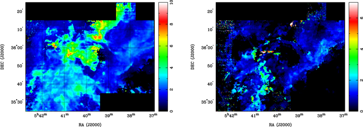
Figure 14. Maps of velocity widths (second moment of the spectrum or dispersion, σV): (left), CO J = 2 − 1 and (right), 13CO J = 2 − 1. Color wedge is in units of km s−1. For a Gaussian line profile, the line FWHM = 2.355 σV. The moment is integrated over the velocity range −28 to −2 km s−1 for both CO and 13CO. Pixels are blanked if the maximum line intensity is less than 0.5 K ( ) in all channels.
Download figure:
Standard image High-resolution image
Figure 15. Distribution of velocity dispersions (second moments, σV) for CO J = 2 − 1 and 13CO J = 2 − 1 maps (see Figure 14). For a Gaussian line profile, the line FWHM = 2.355σV.
Download figure:
Standard image High-resolution image3.6. CO/13CO Ratio Maps and Line Optical Depths
The relative abundance of the CO and 13CO isotopologues is on the order of 50–80 for molecular clouds in the vicinity of the Sun (Milam et al. 2005). Therefore the 13CO line will have a correspondingly lower optical depth compared to the CO line, so even if the CO J = 2 − 1 line is optically thick, the 13CO line may be optically thin, or only marginally thick (τ ≈ 1). If we assume that both isotopologues have similar excitation conditions for the lower rotational levels, and that their relative abundances are constant throughout the cloud, then the observed intensity ratio is a nonlinear function of the CO line optical depth given by
Here the intrinsic ratio of abundances is  , where n(X) is the density of molecular species X. An estimate of the 12C/13C isotope ratio in the interstellar gas at the galactocentric radius of Sh2-235 (∼10.5 kpc) is 80 ± 10 (Milam et al. 2005). Taking f12/13 = 80, the observed line intensity ratio can be used to estimate τCO and
  . For example, a ratio of R = 10 would imply τCO ≈ 8 for the simple homogeneous cloud model. R = 3 gives τCO = 32, and R = 1.58 would imply τCO = 80 and therefore τ13CO ≈ 1, i.e., the 13CO J = 2 − 1 line is becoming optically thick for R ⩽ 1.6.
Figure 16 shows the CO/13CO intensity ratio for selected velocity channels, averaged over 0.45 km s−1, and spaced at 1.35 km s−1 intervals. The "heat" color palette is dark brown at R < 2, indicating very optically thick CO emission, with 13CO becoming moderately optically thick (τ ≳ 1). Positions of the YSOs extracted from the WISE and 2MASS catalogs (Marton et al. 2016—see Section 3.8 below) are marked with symbols indicating the evolutionary class. Generally, the youngest classes, class I and "flat," tend to lie within the high-CO opacity regions at some velocity. For example, note the cluster of class I objects at −16.55 km s−1, associated with the Sh2-235A, B, and C compact H ii regions listed in Table 1.

Download figure:
Standard image High-resolution image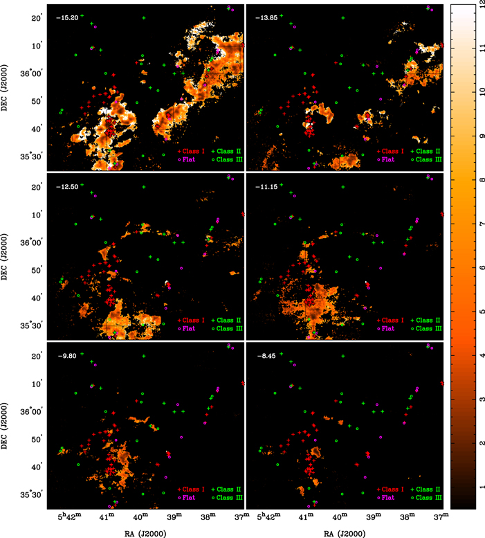
Figure 16. Maps of CO/13CO J = 2 − 1 intensity ratio, averaged over 0.45 km s−1 and spaced 1.35 km s−1 apart. The mean LSR velocity is in the upper left corners of the panels, with the same values as in Figure 10. Color wedge shows the line ratio R as defined in the text. Pixels are blanked if 13CO intensity is < 0.36 K (3 × σ). Symbols mark positions of YSOs, which are distinguished by evolutionary class: red crosses with black outlines are Class I candidates; magenta open circles are "flat" SED sources; green crosses (with black outlines) are class II; green open circles are class III.
Download figure:
Standard image High-resolution image3.7. LTE Analysis
The comparison of the CO J = 3 − 2 and J = 2 − 1 intensities in Figures 5 and 12 indicates that the lower rotational levels of CO are not far from thermal equilibrium. We have therefore analyzed the CO and 13CO J = 2 − 1 maps using an LTE model that assumes that both lines have the same excitation temperature, and that optical depths along each line of sight are in the ratio of the adopted relative abundance of the two isotopologues, namely, CO/13CO = 80 and CO/H2 = 1 × 10⁻⁴. We employed the task colden in the MIRIAD software package (Sault et al. 1995), using as input data the maps of peak CO and 13CO J = 2 − 1 brightness temperature (Figure 3), the 13CO integrated intensity (Figure 6), and the 13CO velocity second moment (Figure 14) multiplied by 2.355 to approximate a Gaussian FWHM. The task produces maps of the CO (and 13CO) excitation temperature, the 13CO optical depth, and the molecular hydrogen column density as outputs. We multiplied the total hydrogen density by 1.40 to correct for He and heavier elements in converting to a total gas column density.
The resulting map of CO (and 13CO) excitation temperature is shown in Figure 17. The bulk of the cloud has temperatures between 10 and 20 K, with smaller regions in excess of 30 K. These warmer areas are mainly associated with gas near the locations of the OB stars, compact H ii regions, and embedded luminous IR sources, marked with white crosses in the figure. The 13CO optical depth distribution is shown in Figure 18. The 13CO optical depth is ⩽1 over most of the map, and exceeds 2 in only a few pixels. We conclude that the 13CO line is not very optically thick anywhere in the cloud, so this basic LTE analysis using the relations plotted in the right panel of Figure 5 is reasonable. The total gas column density from this analysis is given in Figure 19. The total gas mass for the mapped region is 5.2 × 10⁴ M⊙. Because our J = 2 − 1 maps have rms noise levels of ∼0.1 K, even with a 5× rms cutoff in the LTE calculation, the column density map has an excellent dynamic range (≲5–1400 M⊙ pc−2). The distribution is far from uniform, with holes and voids located at the positions of the larger H ii regions (Sh2-231 and -232), and clumpy, high gas column density regions that are evidently associated with ongoing star formation, as indicated by the distribution of YSOs, which are discussed in the next section. It is striking that the 13CO optical depth map (Figure 18) shows a kind of "skeleton" of higher optical depth gas embedded within the relatively uniform excitation temperature map (Figure 17).

Figure 17. Distribution of CO and 13CO J = 2 − 1 excitation temperature, derived by an LTE model (see Section 3.7). Color wedge is in Kelvin, with a square-root stretch to emphasize lower temperature values. The white crosses with black outlines mark the positions of OB stars that ionize H ii regions, and of compact H ii regions or embedded luminous IR sources, as listed in Table 1.
Download figure:
Standard image High-resolution image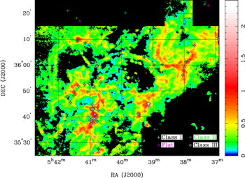
Figure 18. Distribution of 13CO J = 2 − 1 optical depth, derived by an LTE model (see Section 3.7). Color wedge is in nepers of optical depth, with a logarithmic stretch to emphasize low optical depth regions. Colored symbols mark positions of YSOs identified by Marton et al. (2016), which are distinguished by SED classification (see Section 3.8). Note that essentially all pixels have 13CO J = 2 − 1 optical depths <1.5.
Download figure:
Standard image High-resolution image
Figure 19. Distribution of total gas column density, derived by an LTE model (see Section 3.7). The assumed abundance ratios are: CO/H2 = 1E-4 and CO/13CO = 80. The hydrogen column density has been multiplied by a factor of 1.40 to include He and other elements. Color wedge is in M⊙ pc−2, with a logarithmic stretch to emphasize low column density regions. Colored symbols mark the positions of YSOs identified by Marton et al. (2016), which are distinguished by SED classification (see Section 3.8).
Download figure:
Standard image High-resolution imageThe borders of the visible H ii regions are outlined by moderately high gas column densities, which suggests that the expansion of the ionized gas is compressing the molecular cloud where the two gas phases are in contact. This effect is particularly notable around Sh2-231, the large H ii region centered near R.A. 05h39m30s, decl. 35°55'. There is also a prominent ridge of high gas column density that extends some 40' (∼25 pc) along a southeast–northwest line that is roughly tangentential to the shell around Sh2-231. This ridge contains several YSO candidates.
If we employ only an LTE excitation model in this analysis, the J = 2 − 1 transition has the virtue that the line emissivity is relatively insensitive to gas temperature, compared to the J = 1 − 0 or J = 3 − 2 transitions. This lack of strong temperature dependence results from the compensating effects of gas temperature on the line excitation temperature versus the CO partition function. For example, Ginsburg et al. (2011—see their Figure A1) calculate that the total LTE column density derived from a measurement of the 13CO J = 2 − 1 integrated intensity changes by a factor of only 1.25 for excitation temperatures between 10 and 40 K, about the range indicated by our CO J = 2 − 1 peak intensity map for the bulk of the cloud. The line emissivity goes through a shallow minimum at Tex ≈ 17 K (corresponding to the upper state energy, E(J = 2)/k), so the derived LTE column densities are very insensitive to excitation temperature at typical cloud gas kinetic temperatures.
Although this LTE analysis may be a fair representation of the molecular gas distribution in the dense parts of the cloud, an important caveat is the effect of stellar radiation on the gas. The Sh2-235 complex has produced several OB stars, as evidenced by the H ii regions associated with the molecular cloud. These stars must also have an effect on the neutral gas by their UV radiation, which should have created photodissociation (or "photon dominated") regions in the outer parts that surround the dense molecular cores. An analysis of UV radiation effects is beyond the scope of this paper but we will present a more detailed treatment of radiation effects in a future work. It is almost a certainty that in a GMC such as the Sh2-235 complex, there is a substantial amount of mass that is not accounted for by a simple LTE analysis. The masses and gas column densities derived in this section must therefore be considered as only lower limits.
3.8. Comparison with Associated YSOs
Molecular clouds in the galactic anti-center have received relatively less attention in wide-field infrared and submillimeter wavelength studies, compared to regions in the inner Galaxy, or in nearby clouds (d < 1 kpc). As a result, the census of candidate YSOs associated with clouds like the Sh2-235 complex is much less complete than those for regions included in the Spitzer Legacy surveys or the Herschel Key Projects. In recent work utilizing the all-sky infrared surveys of 2MASS (Cutri et al. 2003; Skrutskie et al. 2006) and the WISE satellite (AllWISE, Cutri et al. 2013), Marton et al. (2016) have identified ∼134,000 candidate YSOs over the entire sky. Their analysis uses a support vector machine (SVM) approach, based on artificial intelligence algorithms, to identify candidate YSOs and to differentiate them by spectral class, as an indicator of evolutionary stage. Marton et al. (2016) argue that their method is robust and very effective at rejecting contaminant objects such as external galaxies and galactic red giants (AGB stars), resulting in a clean list of YSO candidates over our CO mapping field. Based on the infrared spectral indices calculated from the 2MASS and WISE data, we use the classifications of Lada (1987) to identify (1) class 0/I (the youngest category, except that we cannot distinguish between the deeply embedded class 0 from class I, so these are lumped together); (2) "flat" SED sources; (3) class II; and (4) class III candidates. We have plotted symbols showing the positions of these four YSO categories in several of the preceding figures, including Figure 6 (CO and 13CO J = 2 − 1 integrated intensity), Figure 7 (CO J = 3 − 2 integrated intensity), and Figure 16 (velocity channel maps of CO/13CO J = 2 − 1 intensity ratio). Figures 6 and 7 show that almost all of the candidate YSOs are found at positions with large CO integrated intensities (in both J = 2 − 1 and 3 – 2 transitions), and most lie on bright 13CO integrated intensities. Figure 19 (LTE-derived gas column density) confirms that most of the youngest YSO classes (class I and "flat") are located at positions of high gas column density. The velocity channel maps of CO/13CO line ratios (Figure 16) allow us to identify the radial velocity of the gas that is associated with the YSOs, and to estimate the CO optical depth at those locations.
The all-sky survey by Marton et al. (2016), however, is limited by the sensitivity of the 2MASS and WISE data. We investigated the limiting magnitudes in the 2MASS J, H, Ks and WISE W1, W2, W3 and W4 bands for the SVM selection method in the entire Sh2-235 complex mapped in CO. Based on the grid of 200,000 YSO models of Robitaille et al. (2006) we estimated the minimum luminosity and mass of a YSO at a distance of 2 kpc that would be classifiable by the SVM method (Marton et al. 2016). The infrared fluxes depend on various other YSO parameters as well, such as the inclination and mass of the protostellar disk and the mass of the envelope around the YSOs. Depending on these parameters, we would be able to identify YSOs with a range of masses and luminosities for a given set of limiting magnitudes. In Table 2 we list the limiting magnitudes for the bands used in our statistical selection of Class I/II and Class III YSOs, and also the masses and luminosities for the faintest YSOs we could reliably classify in the Sh2-235 region. The observations are likely to be biased toward the earlier stages, because the infrared luminosity of the sources decreases with age.
Table 2. Limiting Magnitudes of the Statistical YSO Selection (Marton et al. 2016), and Minimum YSO Mass and Luminosity Detectable at d = 2 kpc
| YSO Class | J | H | KS | W1 | W2 | W3 | W4 | M* | L* |
|---|---|---|---|---|---|---|---|---|---|
| (M⊙) | (L⊙) | ||||||||
| I/II | 17.15 | 15.77 | 15.05 | 14.27 | 14.17 | 10.12 | 7.51 | 0.15 | 0.86 |
| III | 13.53 | 13.14 | 13.02 | 12.86 | 12.59 | 10.37 | 8.18 | 2.1 | 5.9 |
Download table as: ASCIITypeset image
Recent work with JHK band imaging that goes deeper than 2MASS has been published for subsets of the area we mapped in CO, thereby allowing the identification of a more complete list of YSOs, though it was over a more limited spatial extent. A study by Dewangan & Anandarao (2011) of a region ∼20' in size and centered on the Sh2-235 H ii region, combined Spitzer IRAC images together with point-source photometry from ground-based JHK photometric imaging to classify YSOs into class 0/I and class II. Chavarria et al. (2014) analyzed essentially this same region centered on Sh2-235 with the same Spitzer IRAC images but with deeper JHK imaging photometry. Given the deeper near-IR images, they were able to identify about three times as many YSO candidates as Dewangan & Anandarao (2011).
In Figure 20 we show a detail of the 13CO J = 2 − 1 integrated intensity map (from Figure 7, right panel) with the class I YSOs identified by Chavarria et al. (2014) plotted in the left panel and the class II objects in the right panel. The younger class I objects are strongly clustered on the brightest 13CO integrated intensity regions, which also coincide with the Sh2-235 main H ii region and with the group of three compact H ii regions and IR sources, called A, B, and C, that lie ∼8' south of Sh2-235 (see Table 1). The class II objects (right panel of Figure 20), in contrast, are more widely distributed over the region. This greater concentration of the younger class I YSOs on 13CO peaks has been found in many dense young YSO clusters, e.g., in the Serpens cloud (Burleigh et al. 2013).

Figure 20. Detail of the 13CO J = 2 − 1 integrated intensity shown in Figure 7, for a region centered on the Sh2-235 H ii region. The YSO candidates identified by Chavarria et al. (2014) are plotted as white crosses with black outlines: class I (left) and class II (right). White ellipses show possible expansion of a YSO cluster during 2 Myr at a random velocity dispersion of 1.3 km s−1—see Section 5.
Download figure:
Standard image High-resolution imageChavarria et al. (2014) constructed maps of YSO surface density using a variety of spatial-relationship algorithms. In Figure 21 we show their contours of YSO density (in stars pc−2) plotted over the CO J = 2 − 1 peak brightness temperature in the left panel, and over the LTE model-derived total gas column density (in M⊙ pc−2) in the right panel. The highest YSO surface densities generally coincide with the regions of greatest CO J = 2 − 1 brightness temperature and presumably, also the highest gas kinetic temperature. The highest YSO surface densities are also concentrated mainly on the areas with the greatest total gas surface densities.

Figure 21. Detailed maps centered on the Sh2-235 H ii region, of (left) the CO J = 2 − 1 peak brightness temperature (in K), shown in Figure 4; and (right) total gas column density, including He and heavier elements, as derived by our LTE analysis (Section 3.7), in M⊙ pc−2 (see Figure 19). Thick white contours mark gas surface densities of 140 and 500 M⊙ pc−2. The YSO surface density distribution determined by Chavarria et al. (2014) is shown as black contours at 5, 10, 50, and 100 stars pc−2. In the left panel, white crosses mark (from top to bottom) ionizing stars of H ii regions Sh2-235 and Sh2-235A, B, and C (Table 1). The region shown has an area of 125 pc2 and a total gas mass of 19,500 M⊙.
Download figure:
Standard image High-resolution image4. DOWNLOADABLE DATA FILES
The three calibrated brightness temperature image cubes can be downloaded as FITS files using the following links:
- 1.COJ = 2 − 1 FITS files;
- 2.13COJ = 2 − 1 FITS files;
- 3.COJ = 3 − 2 FITS files.
5. DISCUSSION
The main purpose of this article is to present the molecular cloud observations in a variety of formats and to make the calibrated data available as FITS files. In this section, we comment briefly on several points of interest that are already evident in the images, LTE analysis, and related figures presented above.
Evidence for Effects of H iiRegions on Molecular Gas. A comparison of the CO and 13CO maps presented here, with the optical image of the associated H ii regions (see Figure 4 right panel), suggests that the dominant dynamical effect on the molecular gas must be the expansion of the H ii regions that sweeps up and compresses the neutral gas. Ionization of the molecular gas may also play a role but the morphology of the gas column density, as traced in Figure 19 and the CO/13CO line ratios (Figure 16), shows a near-complete absence of CO in the interiors of the largest H ii regions, Sh2-232 and -231, which are partially enclosed by arc-like features with relatively high column density molecular gas. These features are probably portions of swept up material pushed out as the ionized gas expands into the denser but lower pressure neutral cloud. The more optically prominent Sh2-235 H ii region is still partially embedded in the molecular cloud but is evidently beginning to disturb the neutral gas so that it is optically visible, though with spatially non-uniform extinction. The CO velocity dispersion map (Figure 14) shows that the molecular line widths are significantly broadened in the vicinity of Sh2-235, indicating a dynamical interaction. The more compact and embedded Sh2-233 also appears to have begun to compress the molecular gas in its vicinity and possibly to have initiated star formation on the periphery of the ionized gas, as argued by Ladeyschikov et al. (2015).
Triggered Star Formation. Kang et al. (2012) found evidence that the entire Sh2-235 complex has been affected by a supernova remnant (SNR) with an age of ∼0.3 Myr, based on their observations of the H i 21 cm line. Their inferred age, however, is too short for the SNR to have triggered the formation of the ionizing stars in the most extended, oldest of the visible H ii regions, namely Sh2-232, -231, and -235. They speculated that the SNR progenitor was a member of an older cluster in the Aur OB1 association. There appears to be no evidence that the H i shell, evidently driven by the expanding SNR, is directly responsible for the formation of the stars in the Sh2-235 complex.
Kirsanova et al. (2014) made molecular line maps of the ammonia emission in a region of ∼15' × 20' centered on Sh2-235 and -235AB. They compared the gas densities and temperatures for the molecular clumps as derived from the NH3 lines with the requirements of the "collect and collapse" models for the triggered star formation of Whitworth et al. (1994) and concluded that the clusters of YSOs that lie east of the main Sh2-235 H ii region (see Figure 21) could have resulted from the collect and collapse process, provided the density of the gas surrounding the YSO clusters exceeds 3 × 103 cm−3. Our total gas column density map (Figure 21 right panel) for this region shows that these YSO clusters are embedded in high column density clouds. Moreover, the CO J = 3 − 2 maps have strong emission peaks at the positions of the stellar clusters in the velocity range from −18.7 to −16.6 km s−1, shown in Figure 11. At these positions and velocities, the CO (J = 3 − 2)/(J = 2 − 1) intensity ratios approach 1 (Figure 12), indicative of gas volume densities at or above the CO J = 3 − 2 critical density. For a gas temperature of ∼20 K, the J = 3 − 2 critical density is on the order of 1.4 × 104 cm−3 (using a multi-transition definition of critical density,  where the summations in the denominator are over all upward and downward collision rates into the upper level, i.e., u' > u and u > l). Therefore, the physical conditions required for the collect and collapse triggering mechanism to work, according to Kirsanova et al. (2014), appear to be satisfied. Their derived NH3 gas densities are also consistent with the CO J = 3 − 2 critical density needed to excite the observed CO lines.
On a smaller scale, Ladeyschikov et al. (2015) compared the CO and 13CO distributions presented here with the locations and morphologies of IR features in the vicinity of the small H ii region Sh2-233. They concluded that a very red IR source, IRAS 05351+3549, is likely a class 0 YSO, or possibly a pre-stellar core in the process of collapsing under the external pressure of the expanding H ii region, leading to formation of a star. In this object, the mass of material that could be swept up by the expansion of this (young) H ii region is probably too small to explain the estimated clump mass of ∼70 M⊙. The triggered collapse of a pre-existing molecular clump is therefore the more likely mechanism at work.
Distribution of YSOs and Gas Column Density. Several authors have considered the relationship between star formation rates and molecular cloud properties, including gas volume and column densities (Lada et al. 2012; Evans et al. 2014) and cloud structure (Lada et al. 2013). In Figure 22, we compare the distribution functions of the YSO surface density derived by Chavarria et al. (2014) with the gas surface density, Σtotal, which we derived from our LTE analysis of CO and 13CO maps, as described in Section 3.7. The two distributions show significant differences. The YSO surface densities have a nearly exponential distribution above ∼80 stars pc−2, with a cutoff at ∼360 stars pc−2. The distribution rises sharply at low YSO surface density, consistent with the obvious concentration of YSOs at the cloud peaks (Figure 21). In contrast, the gas surface density has a broad maximum between 150–350 M⊙ pc−2, and essentially no pixels below 150 M⊙ pc−2. Above 400 M⊙ pc−2 the hydrogen surface density has a nearly flat plateau, declining slowly out to a sharp cutoff at 950 M⊙ pc−2. Almost every pixel in the left panel of Figure 21 has detectable CO emission, consistent with this portion of the full CO map lying in the center of the Sh2-235 GMC complex.
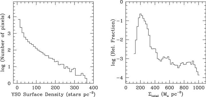
Figure 22. Comparison of YSO and gas surface density distributions for the region shown in Figure 21: (left) YSO surface densities from Chavarria et al. (2014) and (right) total gas surface density, Σtot, (including He) from our LTE analysis of the CO and 13CO J = 2 − 1 maps—see Section 3.7. Note that for a standard gas/dust ratio, 100 M⊙ pc−2 corresponds to 7.0 mag-AV or 0.8 mag-AK.
Download figure:
Standard image High-resolution imageLada et al. (2013) argue that star formation in GMCs occurs only in regions where the K-band extinction exceeds about 0.8 mag. For a standard extinction law (Draine 2011) this value corresponds to AV > 7 mag, and to a total surface density of ∼140 M⊙ pc−2 for a standard gas/dust ratio. Therefore, most of the area shown in Figure 21 has a surface density above the postulated star formation threshold. Comparing the YSO surface density contours with the gas surface density contours in Figure 21 (right panel), it is evident that almost all of the identified YSOs lie within the 140 M⊙ pc−2 contour, consistent with the nominal threshold value. The strongest concentrations (>50 stars pc−2), which define the cluster cores identified by Chavarria et al. (2014), lie within the gas surface density contour at 500 M⊙ pc−2, corresponding to AV > 25 mag.
We also examined the relationship between the total column density derived from our CO and 13CO maps for the region shown in Figure 21, and the surface density of YSOs from Chavarria et al. (2014). In Figure 23 (left panel) we show the average density of YSOs for pixels having Σtotal within bins of width 100 M⊙ pc−2, from 100 to 1000 M⊙ pc−2. The dashed line shows a linear regression fit to a simple power law, with exponent +1.63, with an uncertainty of ±0.2. This slope is in reasonable agreement with that derived by Lada et al. (2013) for the Orion A, California, and Taurus Molecular Clouds, using an entirely different methodology. They inferred Σtotal from their maps of K-band extinction measured for background stars with JHK photometry and applied standard gas-dust ratios and extinction models for the grains. (One caveat in this comparison is that Chavarria et al. (2014) include all IR-excess objects in their YSO density map, i.e., both Class I and Class II, while Lada et al. (2013) consider only the younger Class I sources.)
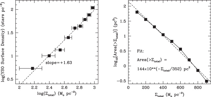
Figure 23. (Left) Dependence of mean YSO surface density on total gas surface density, Σtotal (shown in Figure 21's right panel). The points show values binned between 100 and 200, 200 and 300, etc. M⊙ pc−2. Horizontal bars show the width of each bin. (Right) Cloud area distribution function, i.e., area with surface density ⩾Σtotal. Dashed lines show fits to the points.
Download figure:
Standard image High-resolution image
The area distribution function for the gas surface density map (Figure 21 right panel) is shown in the right side of Figure 23. We plot the total area exceeding Σtotal for each of the nine points, i.e., at 100, 200,..., 900 M⊙ pc−2. Here we find that the area distribution function drops steeply with increasing Σtotal, approximately as an exponential with best-fit parameters given by

where Σtotal is in M⊙ pc2. This functional form is similar to that found by Lada et al. (2013) for the Orion A and Orion B Molecular clouds at the high-extinction end of their graph (see their Figure 6). The central part of the Sh2-235 GMC evidently shows a similar dependence when measured by a completely different method as those found by Lada et al. (2013) from IR extinction data for a different set of GMCs.
Relationship of Cloud Velocity Dispersion to Duration of YSO Evolutionary Stages. The measured 13CO J = 2 − 1 radial velocity dispersion in the areas of highest integrated line intensity in Figure 20 is 1.3 km s−1. If the YSOs being formed in the molecular cloud acquire the same random velocity dispersion, the larger extent of the Class II objects (Figure 20 right) appears to be consistent with the durations of the evolutionary Stages (0+I) and II recommended by Heiderman & Evans (2015), which are ∼0.5 and 2 Myr, respectively. In the left panel of Figure 20 left panel, we show an ellipse of dimensions 4 0 × 11 for the semimajor and semiminor axes, corresponding to 2.3 × 0.64 pc. This ellipse encloses most of the Class I YSOs in the largest young stellar cluster in this region. Assuming that the cloud and star random motions are isotropic, then the observed radial velocity dispersion should equal the dispersion transverse to the line of sight. If the duration of Stage II is 2 Myr and we equate this to the lifetime of YSOs in Class II, and also assume that the currently observed Class II YSOs formed within the same volume as the Class I YSOs, then at 1.3 km s−1, the Class II YSOs would occupy a region larger by 2.7 pc in all directions. The white ellipse in the right panel of Figure 20 illustrates such an expansion to 5.0 × 3.3 pc. Most of the Class II YSOs fall within the expanded ellipse, consistent with most of these stars having formed within a more concentrated volume and having diffused away with a velocity dispersion similar to the molecular gas. Of course, it is not likely that all were in fact formed in the same volume as the stars now identified as Class I, but the relative extent of the two classes as seen in Figure 20, appears to be consistent with such a scenario.
6. SUMMARY
We have presented the results of a program to map the GMC associated with the group of H ii regions cataloged by Sharpless (1959) as Sh2-231, -232, -233, and -235 (collectively called the Sh2-235 molecular cloud complex). The cloud lies in the galactic anti-center at a distance of 2 kpc, placing it in the Perseus spiral arm. It is currently forming numerous stars with spectral types up to O9, within several stellar clusters. We mapped the CO and 13CO J = 2 − 1 transitions using the Heinrich Hertz Submillimeter Telescope, achieving a map resolution of 38'' (FWHM) with an rms noise of 0.12 K main-beam brightness temperature, for a velocity resolution of 0.34 km s−1. With the same telescope, we also mapped the CO J = 3 − 2 line at a frequency of 345 GHz, using a 64-beam focal plane array of heterodyne mixers, achieving a typical rms noise of 0.5 K main-beam brightness temperature with a velocity resolution of 0.23 km s−1 after spatially convolving to an angular resolution of 31''. All the maps were made with the On-The-Fly scanning method, which gives full spatial sampling of the emission. The three spectral line data cubes are available for download (see Section 4).
The data are presented here in several forms, including maps of peak and integrated brightness, as well as of velocity channels spanning the full range of the emission lines. We also show R.A.-velocity maps at selected declinations, and ratio maps of the CO/13CO J = 2 − 1 lines, for representative velocities. The line ratio maps indicate the optical depth of the CO J = 2 − 1 line as a function of spatial position and velocity across the cloud. The ratio of the CO J = 3 − 2 versus J = 2 − 1 brightness temperatures as a function of velocity and position indicates the degree of excitation of the higher-energy J = 3 − 2 line. Much of the cloud appears to be slightly sub-thermally excited in the J = 3 level, except in the vicinity of the warmest and highest column density areas, which are currently forming stars. Using the CO and 13CO J = 2 − 1 lines, we employ an LTE model to derive the gas column density for the entire mapped region.
Comparison of the molecular maps with the locations of H ii regions suggests that expansion of the ionized gas is disrupting the molecular cloud and compressing it at the locations of the YSOs, consistent with a triggering process of star formation. The locations of current star formation in the cloud are concentrated, for the most part, in regions with large gas column density. We compare our CO and 13CO maps with the positions of YSOs cataloged by Marton et al. (2016), as derived from the 2MASS and WISE all-sky surveys. At the distance of the Sh2-235 cloud (2.0 kpc), this catalog of YSOs is complete down to stellar luminosities (listed in Table 2) that depend strongly on the evolutionary class, but are on the order of 1–6 L⊙.
From a deeper survey of YSOs by Chavarria et al. (2014) but restricted to 125 pc2 around the brightest H ii region (Sh2-235), we compare our derived gas column density map with their map of YSO surface density. We find that the YSO surface density scales as a power law of the gas column density with an exponent of 1.6, in reasonable agreement with the results found by Lada et al. (2013) using a different method to derive gas column density. The gas column density area distribution function is well-approximated as an exponential function of the hydrogen column density such that  . The spatial distribution of YSOs of Class 0/I compared with Class II from Chavarria et al. (2014) is consistent with the young stars having the same velocity dispersion as that which we observe in the gas for the highest column density regions, which is where the earliest evolutionary stage YSOs are concentrated. Over a 2 Myr duration the Class II YSOs could have dispersed to their observed spatial extent.
The Heinrich Hertz Submillimeter Telescope is operated by the Arizona Radio Observatory, which is part of Steward Observatory at The University of Arizona. This work was supported in part by National Science Foundation grants AST-0708131 and AST-1140030 to The University of Arizona. We thank Dr. A.R. Kerr of the National Radio Astronomy Observatory for providing the ALMA prototype mixers used in this work. We thank Dr. Luis Chavarria for providing his YSO surface density map in digital form. We also thank the referee, Dr. Peter Barnes, for suggestions that improved this paper.
Footnotes
- 6
The definition of a GMC is somewhat loose, but we follow Draine (2011)—Table 32.2—that GMCs have molecular masses in the range 103–2 × 10⁵ M⊙.
- 7
See the website http://aro.as.arizona.edu/smt_docs/smt_telescope_specs.htm for technical specifications.