


ABSTRACT
We present a new quantitative model for detailed solar-pumped fluorescent emission of the main isotopologue of CN. The derived fluorescence efficiencies permit estimation and interpretation of ro-vibrational infrared line intensities of CN in exospheres exposed to solar (or stellar) radiation. Our g-factors are applicable to astronomical observations of CN extending from infrared to optical wavelengths, and we compare them with previous calculations in the literature. The new model enables extraction of rotational temperature, column abundance, and production rate from astronomical observations of CN in the inner coma of comets. Our model accounts for excitation and de-excitation of rotational levels in the ground vibrational state by collisions, solar excitation to the  and
and  electronically excited states followed by cascade to ro-vibrational levels of
  , and direct solar infrared pumping of ro-vibrational levels in the
  state. The model uses advanced solar spectra acquired at high spectral resolution at the relevant infrared and optical wavelengths and considers the heliocentric radial velocity of the comet (the Swings effect) when assessing the exciting solar flux for a given transition. We present model predictions for the variation of fluorescence rates with rotational temperature and heliocentric radial velocity. Furthermore, we test our fluorescence model by comparing predicted and measured line-by-line intensities for
  (1–0) in comet C/2014 Q2 (Lovejoy), thereby identifying multiple emission lines observed at IR wavelengths.
Export citation and abstract BibTeX RIS
1. BACKGROUND
Comets seem to reveal a complex and dynamic history. Measurements of cometary volatiles have shown a rich chemistry, and new observations continue to add new information that challenges the current understanding of chemical taxonomies and the possible groupings of short- and long-period comets (A'Hearn et al. 1995; Bockelée-Morvan et al. 2004; Mumma & Charnley 2011).
Among molecules surveyed in comets, cyanide was first detected in comet Tebbutt (1881 III) on 1881 June 24 (Huggins 1881) and is one of the most studied molecules in astrophysics (e.g., Ram et al. 2010, and references therein). CN has been characterized in many comets, owing to its relatively long lifetime and unusually strong transitions among its main electronic states ( ,
,  , and
, and  ). The relative abundances of CN, OH, and other free radicals seen at optical wavelengths form the basis for several taxonomic studies of comets based on product species (e.g., A'Hearn et al. 1995; Fink 2009; Schleicher & Bair 2010; Langland-Shula & Smith 2011; Cochran et al. 2012).
The principal electronic transitions of CN are the red (A–X), the violet (B–X), and the LeBlanc (B–A) systems; however, the radiative decay efficiency of the B-state into the A-state is very small compared with decay into the X-state (Cartwright & Hay 1982), and so we omit further consideration of the LeBlanc system from this paper. The (0–0) transitions of the red and violet bands occur near 1100 and 388 nm, respectively.
Observations have provided a wealth of measurements of CN, through the red and violet systems (e.g., Greenstein 1958; Ferrin 1977; Johnson et al. 1983; Schleicher 2010), and the observing strategy and the methodology to analyze these electronic bands of CN isotopologues are well established. Current estimates of CN abundance in comets are based almost entirely on the violet system and indicate that the CN abundance is 0.2%–3.4% relative to OH (Fink 2009; Cochran et al. 2012) with average production rate ratios of 1.7% (Fink 2009). The large survey of 85 comets using narrowband photometry by A'Hearn et al. (1995) found that most CN was produced largely from grains (see also Bonev et al. 2008). Yet, observations at radio and IR wavelengths demonstrate that CN also forms (sometimes mainly; e.g., Gibb et al. 2012) by dissociation of HCN and other primary volatile species in the coma (Bockelée-Morvan & Crovisier 1985; Fray et al. 2005, 2008; Friedel et al. 2005; Cottin & Fray 2008; Paganini et al. 2010, and references therein).
Production rates of cometary HCN are measured directly by observing ro-vibrational transitions at infrared wavelengths and rotational transitions at radio wavelengths and are compared with CN production rates obtained at optical wavelengths. However, direct comparisons are often limited by intrinsic properties pertaining to the observing characteristics, such as different fields of view (FOVs) and the different excitation mechanisms at work. Indeed, comparative analyses of relative abundances of primary and product species (e.g., HCN/H2O and CN/OH) can be problematic because optical observations measure by-products (e.g., CN) of primary volatiles (e.g., HCN) or dust grains, but they do not identify or measure the primary source species itself (cf. Fray et al. 2005; Bonev et al. 2008; Mumma & Charnley 2011; Gibb et al. 2012). When present in the coma, extended sources of these molecules (e.g., Cottin & Fray 2008) add another source of uncertainties (e.g., Feldman et al. 2015). The complex parameters pertaining to the excitation and chemical (photodissociation) processes in the outer coma differ greatly from those observed in the close nucleus environment, and emissions contributed from these regions can yield different results for production rates (e.g., see Figure 5 in Combi et al. 2013).
Schleicher (2010) reviewed several models used to estimate CN production rates in comets, beginning with that of Tatum & Gillespie (1977)—the first general solution developed for extracting the CN column density from the integrated intensity of the violet (0–0) band emission as a function of heliocentric distance. Soon after, Mumma et al. (1978) developed a model for line-by-line fluorescence intensities using a full-disk model for solar irradiance (results are shown in A'Hearn 1982), and Schleicher (1983) and Tatum (1984) later developed similar models. Danks & Arpigny (1973) studied the relative band intensities of the CN red and violet systems without including the rotational structure, and Fink (1994) did so for the red system. Zucconi & Festou (1985) computed a complete fluorescence spectrum of the CN radical, taking into account the rotational structure of both the red and violet systems, and Kleine et al. (1994) computed rotational line fluorescence efficiencies for stable isotopologues of CN (12C14N, 13C14N, and 12C15N), including the effects of collisions as an alternative excitation mechanism, secondary to fluorescence.
In the near-IR (NIR), high-resolution spectroscopy can attain detections of CN emission lines of the  (1–0) band, around 2055 cm−1 (or 4866 nm). The CN (1–0) R3 line near 2057 cm−1 (or 4861 nm) was first detected serendipitously during searches for OCS in C/1996 B2 (Hyakutake) and C/1995 O1 (Hale-Bopp); Dello Russo et al. 1998), yet the lack of fluorescence efficiencies has precluded the extraction of CN column densities and production rates within the coma and limited the IR study of this product volatile and its role within the NIR chemical taxonomy of comets. Most of these limitations stem from the lack of theoretical and laboratory data and from the need to calculate multiband excitation and cascade within the combined CN band systems (B–X, A–X, and X–X). We tackle these limitations in this study. Recently, Brooke et al. (2014) published Einstein coefficients and line strengths for many bands of the
  –
– and
and  –
– electronic systems and for ro-vibrational transitions within the
  state of CN; however, they did not calculate fluorescence efficiencies for realistic cometary conditions.
We have developed a model that provides calculations of fluorescence efficiencies (also called g-factors) for ro-vibrational transitions in the ground electronic state of the main CN isotopologue (12C14N), as well as for lines from A–X and B–X bands observed at shorter wavelengths. We include fluorescent pumping from X2Σ+ to the higher electronic states (namely, A2Πi and B2Σ+) and trace the subsequent cascade into the ground electronic level (X2Σ+).
Our calculations will allow existing and future observers to identify and quantify CN radicals in cometary exospheres (comae), simultaneously with other important volatiles such as H2O and CO, thus permitting the comparison of rotational temperatures and column densities for these species, from which production rates and relative abundance ratios can be obtained using appropriate dynamical models. Ultimately, this will permit us to enhance the current understanding of CN origins and chemistry.
We recently detected CN (X2Σ+, 1–0) emission lines in comet C/2014 Q2 (Lovejoy) near 4.9 μm (L. Paganini et al. 2016, in preparation). Our observations featured simultaneous detection of emission lines from CN, OCS, and H2O (see Section 3). The partial overlapping of some of these lines (mainly CN and OCS) and the aforementioned need for detailed fluorescence efficiencies in the NIR motivated the present work.
2. METHODOLOGY
Herzberg (1950) described the quantum structure of diatomic molecules including CN, while Kleine et al. (1994) and Aikman et al. (1974) provide good summaries of the main characteristics for CN. Rotational states of CN are identified by the rotational quantum number (N), the total angular momentum (J), and the parity of the state (+ or −). Each rotational level (except N = 0, for 2Σ states) in a given vibrational level (v) splits into a spin doublet (F1 and F2 levels), where F1 levels correspond to J = N + 1/2 and the F2 levels to J = N − 1/2. In the A2Π state, each J-value splits further into two levels due to Λ-doubling.
We computed pumping efficiencies by solar excitation from X2Σ+ (v'' = 0) into levels of the A2Π and B2Σ+ states followed by radiative decay into ro-vibrational levels of X2Σ+ again, and also for direct solar pumping at infrared wavelengths among levels of the X state alone. We considered 40 rotational levels within 15 vibrational states for each electronic configuration (B, A, and X) and accounted for both resonant and nonresonant fluorescence (the latter into v''  0). The modeled products are fluorescence efficiencies for individual spectral lines in the ro-vibrational emission spectrum of the B, A, and X combination band systems of CN.
As in the case of OH prompt emission from photolysis of H2O, we expect to detect certain emissions that cannot be pumped efficiently by solar fluorescence alone (Mumma et al. 2001; Bonev et al. 2004, 2006; Bonev & Mumma 2008). Bodewits et al. (2016) discuss that photodissociation of HCN is not a very efficient mechanism for producing prompt emission from CN (Bockelée-Morvan & Crovisier 1985; Fray et al. 2005), and they suggest that electron impact dissociation of HCN likely drives the production of excited CN instead. This suggestion triggers the need for further studies to seek prompt emission of CN in comets to test its possible precursors, yet the lack of sufficient laboratory measurements forbids inclusion of such treatment in this paper.
The computation of CN g-factors consists of three stages: (1) estimating the rotational population in the ground vibrational level, (2) calculating the pumping coefficients using a reliable solar spectrum, and (3) determining the radiative decay. We next describe these steps.
2.1. Rotational Populations
In a multilevel system, the line transfer between molecular ro-vibrational levels, u (upper) and l (lower), is determined by transition rates appropriate to their specific populations, nu and nl. This transfer involves collisional and radiative processes and is commonly described by the statistical equilibrium (SE) equation:
where Rul and Rlu are the rate coefficients for loss from and entry into level u, respectively, resulting from collisions (both exciting and de-exciting), absorption of photons (excitation), and stimulated and spontaneous emission (de-excitation). External effects include solar and cosmic microwave background (CMB) radiation and local excitation caused by electron and neutral collisions. We defer consideration of thermal emission from dust and the comet nucleus to a future publication.
Schleicher (2010) discusses the omission of key vibrational and electronic levels to explain the mismatch of models and astronomical measurements for the violet system and cites the minor role of collisions in fluorescent equilibrium models (e.g., based on studies by Arpigny 1964 and Ishii & Tamura 1979). However, care must be taken in some specific cases. Collisions shape rotational populations in the ground vibrational state in the inner coma, where neutral gas density exceeds the critical density (whose value depends on water production rates, thermal and outflow velocities, and the molecular transition under consideration; Weaver & Mumma 1984; Xie & Mumma 1992; Bensch & Bergin 2004; Zakharov et al. 2007). At greater nucleocentric distances, collisions become less important and rotational populations increasingly approach fluorescence equilibrium. Observations taken with a large FOV tend to reflect the latter condition, but observations of the mid- and near-nucleus coma taken with a small FOV (e.g., most NIR observations, or near-nucleus observations by spacecraft) are dominated by collisions with neutrals (mainly H2O, CO, and CO2) and with electrons (details depend on production rates and other parameters; e.g., Feldman et al. 2015)—each situation must be considered on a case-by-case basis. These different processes and environments can be treated with the radiative transfer (RT) and SE equations.
The RT equation describes the emission and scattering of photons along a line in the direction of propagation (see van der Tak et al. 2007, for further details) and is defined as

where  is the source function,
  represents the specific intensity of electromagnetic radiation, and
  ds is the optical depth, with the source function Sul(ν) depending on the emission εul(ν) and absorption αij(ν) coefficients as Sul(ν) = εul(ν)/αul(ν). These coefficients are defined by


These equations involve Einstein coefficients for spontaneous emission and absorption, Aul and Blu, and for stimulated emission, Bul. Brooke et al. (2014) published Einstein coefficients and line strengths for many bands of the A2Π–X2Σ+ and B2Σ+–X2Σ+ electronic systems and for ro-vibrational transitions within the X2Σ+ state of CN (they used the pgopher program of Western 2010), and they considered the J dependence of the transition dipole moment matrix elements—the Herman–Wallis effect (see their paper for further details).
Collisional processes are defined by the rate Cul = ncpkul, with kul being the collisional rate coefficient and ncp the density of the collision partner(s). For our model, we considered collisions of CN with electrons (e–, hereafter e) and water (we defer the consideration of diverse molecular collision partners to a future paper). We obtained detailed e-CN cross sections from the Leiden Atomic and Molecular Database3 and scaled the electron density and temperature profiles from measurements in the coma of 1P/Halley, following the approach advocated by Biver (1997) (see also Xie & Mumma 1992).
Since detailed CN–H2O cross sections are not yet available, we followed the standard procedure of assuming a constant cross section that is independent of relative velocity and ro-vibrational transition, equal to 40 Å2 (or 4 × 10⁻¹⁵ cm2; Kleine et al. 1994), corresponding to a collision rate of 1.93 × 10⁻¹⁰ cm3 s−1 at an assumed kinetic temperature of 100 K. As noted by Kleine et al., this value could be larger due to the long-range interaction between polar molecules (Green 1985).
Assuming spherically symmetric release from the nucleus and uniform outflow velocity, the density distribution of primary water can be estimated using a quantitative description presented by Haser (1957):

where ρ is the nucleocentric distance (radius), vexp is the expansion velocity, and λp is the photodissociation scale length equal to vexp/β, where the photodissociation rate is β0 at 1 AU and scales as  . We took the lifetime-defining photodissociation rate coefficients (β0) from Huebner et al. (1992). Equation (5) is based on several simplifying assumptions; for example, it omits the increase in expansion velocity with nucleocentric distance, assumes kinetic velocities to be constant, and omits H2O release from icy-mantled grains in the near-nucleus coma region.
The origin of cometary CN radicals is a subject of extensive debate (e.g., Fray et al. 2005), and its roots are reviewed and discussed in Paganini et al. (2010). HCN is a known source of CN in cometary exospheres. Photodissociation of HCN leads to direct formation of H and CN, with a branching ratio of 97% (Huebner et al. 1992), and the production rates of HCN and CN are consistent in some comets. However, the production rate of CN often greatly exceeds the production rate of HCN, demonstrating that other production mechanisms are present; dust grains were identified as the principal precursor of CN in the study of 85 comets by A'Hearn et al. (1995), but see the earlier discussion in Section 1.
With the assumption of a single gaseous precursor (HCN), the density of CN is defined by

If written in the form of modified Bessel functions, Equation (6) becomes
where K0(y) is the modified Bessel function of the first kind (Combi et al. 2004 and references cited therein).
This system of linear equations is handled by the public version of an RT code Radex (van der Tak et al. 2007), which uses a treatment of optical depth effects based on an escape probability method. The key inputs to Radex are (1) frequency range for the calculation (GHz), (2) kinetic temperature of the coma (K), (3) number of collision partners (we chose H2O and e), (4) density of collision partners, (5) temperature of the CMB (2.73 K), (6) the column density of CN, and (7) the FWHM line widths of CN spectral lines. The solution ultimately yields the level populations of CN in the ground vibrational level, at the corresponding nucleocentric distances.
If we assume thermodynamic equilibrium, the rotational level population in the ground vibrational state is defined by a Boltzmann distribution, simplifying the computational leverage. This assumption is valid for most cases in the NIR, if the FOV encompasses distances where collisions with water are the dominant excitation mechanism; however, in the electron collision zone (between the contact and recombination surfaces, Rcs and Rrec; cf. Gombosi 2015) level populations change slightly, ultimately producing variations in estimated g-factors. Table 1 shows a comparison of the relative populations obtained, for two cases: (1) assuming a Boltzmann distribution and (2) assuming different FOV radii using Radex (see also Figure 1). The ends of our 1 78 long NIRSPEC slit extract correspond to a cometocentric distance of ∼645 km at the tangent point along the line of sight (typical for our extraction with Keck-2/NIRSPEC); the 2000 km distance corresponds to the region where electrons dominate excitations (between Rcs and Rrec) in our test case (i.e., a comet at heliocentric (Rh) and geocentric (Δ) distances of 1 AU; see Figure 1). We observe odd–even variations, which depend on the spin statistics (degeneracy) and energy levels of each particular rotational level.
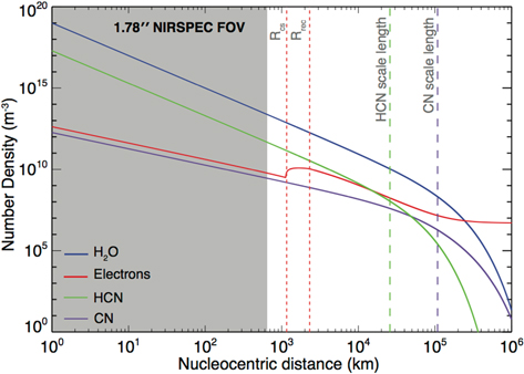
Figure 1. Coma density profile of key species in our model. The shaded region represents the range of nucleocentric distance sampled in our model. These values serve as input parameters for the radiative transfer model (Radex) and are used to identify the excitation conditions of given astronomical observations. In this example we consider HCN/H2O = 0.2%, Rh = Δ = 1 AU, Q(H2O) = 1 × 1029 s−1, vexp = 0.8 Rh , βH2O = 1.5 × 10⁻⁵ s−1, βHCN = 3.1 × 10⁻⁵ s−1, and βCN = 7.4 × 10⁻⁶ s−1 (for active Sun, after Huebner et al. 1992), and thus
  = 2.6 × 10⁴ km,
  = 1.1 × 10⁵ km. We typically use a NIRSPEC footprint of 042 × 178 for nucleus-centered extracts of molecular emissions; at 1 AU from Earth the length spans a cometocentric distance of ±645 km at the tangent point (shaded region). The electron collision zone (between the contact and recombination surfaces, Rcs and Rrec) lies well beyond the inscribed sphere of 645 km radius, in this test case. However, it can still be important—with a production scale length exceeding many thousand kilometers, most CN lies well outside the inscribed sphere and within the electron collision zone. See Section 2.1 for further details.
Download figure:
Standard image High-resolution imageTable 1. Level Population (Pj) of the Ground Vibrational Level of the X2Σ+ Band, Assuming a Test Case of a Comet with Q(H2O) = 1E29 s−1, Located at Rh = Δ = 1 AU
| Rotational Temperature | |||||||
|---|---|---|---|---|---|---|---|
| N'' | J'' | 50 K | 100 K | ||||
| Boltzmann | Nucleocentric Distance | Boltzmann | Nucleocentric Distance | ||||
| 645 km | 2000 km | 645 km | 2000 km | ||||
| 0 | 0.5 | 0.05343 | 0.05350 | 0.05480 | 0.02696 | 0.02700 | 0.02750 |
| 1 | 0.5 | 0.04793 | 0.04800 | 0.04930 | 0.02553 | 0.02560 | 0.02610 |
| 1 | 1.5 | 0.09583 | 0.09610 | 0.09930 | 0.05106 | 0.05120 | 0.05290 |
| 2 | 1.5 | 0.07712 | 0.07750 | 0.08000 | 0.04580 | 0.04600 | 0.04800 |
| 2 | 2.5 | 0.11562 | 0.11600 | 0.12100 | 0.06868 | 0.06910 | 0.07300 |
| 3 | 2.5 | 0.08347 | 0.08400 | 0.08660 | 0.05836 | 0.05880 | 0.06270 |
| 3 | 3.5 | 0.11121 | 0.11200 | 0.11600 | 0.07778 | 0.07850 | 0.08490 |
| 4 | 3.5 | 0.07202 | 0.07240 | 0.07350 | 0.06259 | 0.06330 | 0.06830 |
| 4 | 4.5 | 0.08994 | 0.09060 | 0.09240 | 0.07820 | 0.07920 | 0.08650 |
| 5 | 4.5 | 0.05225 | 0.05220 | 0.05110 | 0.05961 | 0.06030 | 0.06450 |
| 5 | 5.5 | 0.06263 | 0.06270 | 0.06160 | 0.07149 | 0.07250 | 0.07830 |
| 6 | 5.5 | 0.03264 | 0.03230 | 0.02970 | 0.05161 | 0.05210 | 0.05380 |
| 6 | 6.5 | 0.03803 | 0.03760 | 0.03470 | 0.06017 | 0.06080 | 0.06330 |
| 7 | 6.5 | 0.01778 | 0.01730 | 0.01450 | 0.04115 | 0.04130 | 0.03980 |
| 7 | 7.5 | 0.02029 | 0.01970 | 0.01660 | 0.04699 | 0.04720 | 0.04580 |
| 8 | 7.5 | 0.00851 | 0.00805 | 0.00593 | 0.03043 | 0.03020 | 0.02640 |
| 8 | 8.5 | 0.00956 | 0.00905 | 0.00670 | 0.03421 | 0.03400 | 0.02990 |
| 9 | 8.5 | 0.00360 | 0.00330 | 0.00208 | 0.02099 | 0.02050 | 0.01580 |
| 9 | 9.5 | 0.00399 | 0.00366 | 0.00231 | 0.02330 | 0.02270 | 0.01760 |
| 10 | 9.5 | 0.00135 | 0.00119 | 0.00063 | 0.01354 | 0.01290 | 0.00868 |
| 10 | 10.5 | 0.00148 | 0.00131 | 0.00069 | 0.01488 | 0.01420 | 0.00955 |
Download table as: ASCIITypeset image
The values given in Table 1 differ from those of Schleicher (2010), who assumed fluorescence equilibrium. This difference is expected when different excitation mechanisms drive the excitation (collisions versus fluorescence equilibrium). The distribution of rotational levels (characterized by Trot; see Equations (8) and (9) in Section 2.2) directly impacts the estimated fluorescence rates (g-factors). In Section 2.2 we provide the resulting g-factors, and in Section 2.3 we present comparisons with previous computations.
2.2. Excitation and Fluorescence Rates
The determination of g-factors has been broadly explained in the literature, so we give only a short overview here (see Crovisier & Encrenaz 1983; Weaver & Mumma 1984; Zucconi & Festou 1985; Bockelée-Morvan 1987, for further details). Using level populations obtained for the lower energy levels (Pj described in Section 2.1), we estimate the direct pumping rates (g-factor, photons molecule−1 s−1) resulting from solar infrared irradiation, using
where wl and wu are the lower- and upper-level statistical weights, respectively, νul is the frequency, and J(νul) is the solar flux density.
We remind the reader that the Swings effect is considered in our models, but not until Section 2.4 do we analyze the effect of heliocentric velocity. Prior to Section 2.4, g-factors consider a heliocentric velocity ( ) of 0 km s−1.
Fluorescence excitation depends strongly on variations of solar radiation with wavelength, which are strong in the CN band systems owing to the high abundance of CN in the solar atmosphere. Using an accurate estimate of the solar flux is key for accurate determinations of the excitation process. We generated disk-averaged solar spectra by combining data from the Atmospheric Chemistry Experiment (ACE) and a purely theoretical model (Kurucz 1997). We followed the synthetic methodology described in Villanueva et al. (2011), where our hybrid model convolves the generated disk-averaged solar spectra with a modeled limb-darkening profile. The ACE spectrum features very high resolving power (v/δv ∼ 1 × 10⁵ from 750 to 4400 cm−1; Hase et al. 2010), spanning most of the X–X band system, while the theoretical model covers the A–X and B–X band systems. Examples of the convolved spectra are shown in Figure 2; Fraunhofer lines of solar CN (X2Σ+—X2Σ+) are shown as an inset.
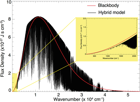
Figure 2. Comparison of the expected solar flux density at the top of the atmosphere from our hybrid model and a typical blackbody at 5770 K. An accurate estimate of the solar flux is key for accurate determinations of the excitation process. Inset: region covering the X (1–0) band. See Section 2.4 for further details.
Download figure:
Standard image High-resolution imageUsing Equation (8), we estimate the effective (excitation) pumping rate of rotational levels in v'' = 0 by direct infrared pumping. Later on, we estimate the radiative decay from excited ro-vibrational levels in higher vibrational states (v' = 1, 2, 3, ...15), including excitation and cascade from B and A electronic states into X-state ro-vibrational levels (to account for nonresonant fluorescence), following selection rules and Equation (9), described next.
For CN, the selection rules governing electric dipole transitions require that ΔJ = J' − J'' = 0, ±1, and the parity of the states involved in the transitions must change. For transitions involving 2Σ–2Σ levels, there is an additional selection rule: ΔN = ±1, and ΔJ = 0 is strictly forbidden. For them (e.g., B–X and X–X), there is no Q-branch, and the band system is characterized by R- and P-branches corresponding to transitions ΔJ = +1 and ΔJ = −1, respectively. The effect of these selection rules requires three components for each spectral line: R1, R2, and satellite transition RQ21  , or P1, P2, and PQ12 shown in Figure 3.
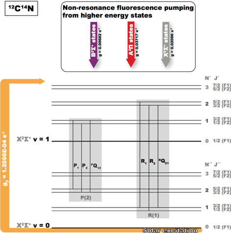
Figure 3. Example of ro-vibrational transitions in the v'−v'' = (1–0) system of the X2Σ+ band, characterized by hyperfine structures (Px, Rx, and satellite transitions PQx and RQx) that form the resulting lines in the P- and R-branches. The hyperfine structures are displayed in shaded gray. The contribution from upper levels to v'' = 1 is shown in the inset "Non-resonance fluorescence pumping from higher energy states." A large contribution comes from the higher cascading X-vibrational states and the red and violet bands. For these calculations we assume Rh = 1 AU and  km s−1.
Download figure:
Standard image High-resolution imageOnce fluorescence is traced, we estimate the detailed cascading fluorescence rate for each ro-vibrational level using

In Table 2, we provide a list of g-factors at Rh = 1 AU, supposing the following: pure excitation of ro-vibrational transitions in X2Σ+ by solar flux alone (see note "a" in Table 2), and excitation of ro-vibrational transitions in X2Σ+ including the pumping contribution from the B–X and A–X systems (see note "b" in Table 2). The net result demonstrates that optical pumping through the red and violet bands is responsible for a significant fraction of the predicted fluorescent intensity in the CN (1–0) band.
Table 2.
Fluorescence Efficiencies (g-factor) of Ro-vibrational Transitions (P1–P7, R0–R5) in the X2Σ+ (1–0) Band Considering Solar Flux Only versus Pumping from the B–X and A–X Band Systems, Assuming Rh = 1 AU and  km s−1
| WN | El | E' | v' | E'' | v'' | N' | J' | p | N'' | J'' | p | Description | ga | gb |
|---|---|---|---|---|---|---|---|---|---|---|---|---|---|---|
| 2015.2192 | 105.9 | X | 1 | X | 0 | 6 | 6.5 | 1e | 7 | 7.5 | 1e | pP1(7.5) | 1.29E−06 | 1.15E−03 |
| 2015.2269 | 105.9 | X | 1 | X | 0 | 6 | 5.5 | 2f | 7 | 6.5 | 2f | pP2(6.5) | 1.13E−06 | 1.56E−03 |
| 2015.2736 | 105.9 | X | 1 | X | 0 | 6 | 6.5 | 1e | 7 | 6.5 | 2f | pQ12(6.5) | 1.29E−08 | 1.15E−05 |
| 2019.2072 | 79.4 | X | 1 | X | 0 | 5 | 5.5 | 1e | 6 | 6.5 | 1e | pP1(6.5) | 2.39E−06 | 1.80E−03 |
| 2019.2149 | 79.4 | X | 1 | X | 0 | 5 | 4.5 | 2f | 6 | 5.5 | 2f | pP2(5.5) | 2.02E−06 | 2.28E−03 |
| 2019.2544 | 79.4 | X | 1 | X | 0 | 5 | 5.5 | 1e | 6 | 5.5 | 2f | pQ12(5.5) | 3.21E−08 | 2.42E−05 |
| 2023.1614 | 56.7 | X | 1 | X | 0 | 4 | 4.5 | 1e | 5 | 5.5 | 1e | pP1(5.5) | 2.63E−06 | 2.70E−03 |
| 2023.169 | 56.7 | X | 1 | X | 0 | 4 | 3.5 | 2f | 5 | 4.5 | 2f | pP2(4.5) | 2.16E−06 | 3.02E−03 |
| 2023.2013 | 56.7 | X | 1 | X | 0 | 4 | 4.5 | 1e | 5 | 4.5 | 2f | pQ12(4.5) | 5.02E−08 | 5.14E−05 |
| 2027.0814 | 37.8 | X | 1 | X | 0 | 3 | 3.5 | 1e | 4 | 4.5 | 1e | pP1(4.5) | 3.16E−06 | 3.15E−03 |
| 2027.089 | 37.8 | X | 1 | X | 0 | 3 | 2.5 | 2f | 4 | 3.5 | 2f | pP2(3.5) | 2.45E−06 | 3.18E−03 |
| 2027.1141 | 37.8 | X | 1 | X | 0 | 3 | 3.5 | 1e | 4 | 3.5 | 2f | pQ12(3.5) | 9.24E−08 | 9.22E−05 |
| 2030.9672 | 22.7 | X | 1 | X | 0 | 2 | 2.5 | 1e | 3 | 3.5 | 1e | pP1(3.5) | 4.01E−06 | 3.61E−03 |
| 2030.9747 | 22.7 | X | 1 | X | 0 | 2 | 1.5 | 2f | 3 | 2.5 | 2f | pP2(2.5) | 2.76E−06 | 3.01E−03 |
| 2030.9926 | 22.7 | X | 1 | X | 0 | 2 | 2.5 | 1e | 3 | 2.5 | 2f | pQ12(2.5) | 2.04E−07 | 1.84E−04 |
| 2034.8187 | 11.4 | X | 1 | X | 0 | 1 | 1.5 | 1e | 2 | 2.5 | 1e | pP1(2.5) | 3.44E−06 | 2.96E−03 |
| 2034.8261 | 11.3 | X | 1 | X | 0 | 1 | 0.5 | 2f | 2 | 1.5 | 2f | pP2(1.5) | 1.92E−06 | 1.85E−03 |
| 2034.8368 | 11.3 | X | 1 | X | 0 | 1 | 1.5 | 1e | 2 | 1.5 | 2f | pQ12(1.5) | 3.88E−07 | 3.34E−04 |
| 2038.6356 | 3.8 | X | 1 | X | 0 | 0 | 0.5 | 1e | 1 | 1.5 | 1e | pP1(1.5) | 7.78E−07 | 2.03E−03 |
| 2038.6465 | 3.8 | X | 1 | X | 0 | 0 | 0.5 | 1e | 1 | 0.5 | 2f | pQ12(0.5) | 3.92E−07 | 1.02E−03 |
| 2046.1615 | 0 | X | 1 | X | 0 | 1 | 0.5 | 2f | 0 | 0.5 | 1e | rQ21(0.5) | 9.85E−07 | 9.49E−04 |
| 2046.1722 | 0 | X | 1 | X | 0 | 1 | 1.5 | 1e | 0 | 0.5 | 1e | rR1(0.5) | 1.99E−06 | 1.71E−03 |
| 2049.8666 | 3.8 | X | 1 | X | 0 | 2 | 1.5 | 2f | 1 | 1.5 | 1e | rQ21(1.5) | 3.19E−07 | 3.48E−04 |
| 2049.8775 | 3.8 | X | 1 | X | 0 | 2 | 1.5 | 2f | 1 | 0.5 | 2f | rR2(0.5) | 1.61E−06 | 1.75E−03 |
| 2049.8845 | 3.8 | X | 1 | X | 0 | 2 | 2.5 | 1e | 1 | 1.5 | 1e | rR1(1.5) | 2.98E−06 | 2.68E−03 |
| 2053.5365 | 11.4 | X | 1 | X | 0 | 3 | 2.5 | 2f | 2 | 2.5 | 1e | rQ21(2.5) | 1.29E−07 | 1.69E−04 |
| 2053.5546 | 11.3 | X | 1 | X | 0 | 3 | 2.5 | 2f | 2 | 1.5 | 2f | rR2(1.5) | 1.84E−06 | 2.39E−03 |
| 2053.5616 | 11.4 | X | 1 | X | 0 | 3 | 3.5 | 1e | 2 | 2.5 | 1e | rR1(2.5) | 2.64E−06 | 2.64E−03 |
| 2057.1711 | 22.7 | X | 1 | X | 0 | 4 | 3.5 | 2f | 3 | 3.5 | 1e | rQ21(3.5) | 6.65E−08 | 9.29E−05 |
| 2057.1965 | 22.7 | X | 1 | X | 0 | 4 | 3.5 | 2f | 3 | 2.5 | 2f | rR2(2.5) | 1.83E−06 | 2.55E−03 |
| 2057.2034 | 22.7 | X | 1 | X | 0 | 4 | 4.5 | 1e | 3 | 3.5 | 1e | rR1(3.5) | 2.38E−06 | 2.43E−03 |
| 2060.7703 | 37.8 | X | 1 | X | 0 | 5 | 4.5 | 2f | 4 | 4.5 | 1e | rQ21(4.5) | 4.10E−08 | 4.62E−05 |
| 2060.8029 | 37.8 | X | 1 | X | 0 | 5 | 4.5 | 2f | 4 | 3.5 | 2f | rR2(3.5) | 1.85E−06 | 2.08E−03 |
| 2060.8097 | 37.8 | X | 1 | X | 0 | 5 | 5.5 | 1e | 4 | 4.5 | 1e | rR1(4.5) | 2.28E−06 | 1.72E−03 |
| 2064.3338 | 56.7 | X | 1 | X | 0 | 6 | 5.5 | 2f | 5 | 5.5 | 1e | rQ21(5.5) | 1.63E−08 | 2.26E−05 |
| 2064.3737 | 56.7 | X | 1 | X | 0 | 6 | 5.5 | 2f | 5 | 4.5 | 2f | rR2(4.5) | 1.09E−06 | 1.51E−03 |
| 2064.3804 | 56.7 | X | 1 | X | 0 | 6 | 6.5 | 1e | 5 | 5.5 | 1e | rR1(5.5) | 1.29E−06 | 1.15E−03 |
Notes. WN: wavenumber (cm−1); g: g-factor (photons molecule−1 s−1); El: lower energy level (cm−1); E: electronic level; v: vibrational level; N: rotational quantum number; J: total angular momentum; p: parity. Note that ' and '' indicate upper and lower levels, respectively. This nomenclature is standard among the molecular community (e.g., Brooke et al. 2014).
aAssuming pure excitation of ro-vibrational transitions by solar flux alone. bg-factors for ro-vibrational transitions after including the pumping contribution from the B–X and A–X band systems. The B–X and A–X terms dominate the X–X pumping by 3 orders of magnitude.Download table as: ASCIITypeset image
We emphasize direct excitation and decay among ro-vibrational levels within the X-state alone and radiative pumping and decay from the A and B states. In Tables 3–4 and Figure 4, we show an example of the contribution (i.e., branching ratios, percentage) from the lower three vibrational states in the A- and B-states to the X-state. The g-factors from the main bands of CN resulting from our full-band model are displayed in Figure 5. In Figure 6 we show an expanded view of the infrared ro-vibrational emission bands: (1–0), (2–1), and (3–2) near 5 μm. A complete listing of line-by-line g-factors, including for the B–X and A–X band systems, can be provided by the authors upon request.

Figure 4. CN full-band fluorescence model. Solar excitation and cascading from ro-vibrational lines in the B2Σ+ and A2Π levels and contributions (i.e., branching ratios, %) to the X2Σ+ ro-vibrational lines. For simplicity, we show the lowest four vibrational levels in each electronic energy state. For these calculations we assume Rh = 1 AU and  km s−1.
Download figure:
Standard image High-resolution image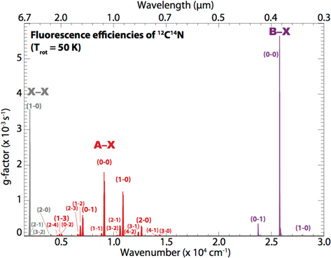
Figure 5. Fluorescence efficiencies of the most important (B–X), (A–X), and (X–X) band systems of 12C14N. Efficiencies around 2050 cm−1 are strong and allow sensing of 12C14N at IR wavelengths. They largely reflect the very large g-factors for the red (A–X) and violet (B–X) systems that produce efficient vibrational excitation in the X-state. The x-axis extends from 1500 cm−1 (6.7 μm) to 30,000 cm−1 (0.3 μm). The (X, 1–0) band is at 2050 cm−1 (4.9 μm), highlighted in Figure 6. For these calculations we assume Rh = 1 AU and  km s−1.
Download figure:
Standard image High-resolution image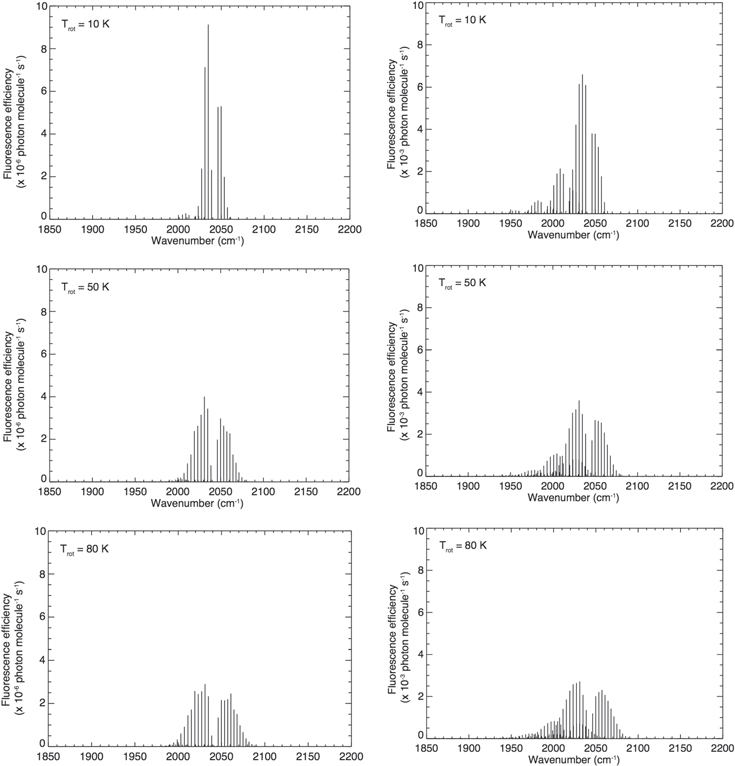
Figure 6. Fluorescence efficiency of the (1–0) system. Left: direct pumping within X2Σ+ only (pumping from the B and A states is omitted). Right: same after considering cascading from the B–X and A–X bands. The contribution from these higher electronic levels (Figure 3) yields strong fluorescence pumping into the (1–0) system, about 3 orders of magnitude stronger than direct pumping within the X2Σ+ state alone. Cascade also pumps significant hot-band emission (2–1 and 3–2). We assume Rh = 1 AU and  km s−1.
Download figure:
Standard image High-resolution imageTable 3. Calculated Branching Ratios (%) of the (v'−v'') CN Red System (see Figure 4)
| v''\v' | 0 | 1 | 2 | 3 |
|---|---|---|---|---|
| 0 | 73.2 | 73.6 | 42.1 | 18.3 |
| 1 | 24.2 | 4.9 | 44.3 | 53.8 |
| 2 | 2.5 | 17.5 | 1.3 | 14.7 |
| 3 | ∼0 | 3.7 | 8.3 | 7.3 |
Note. Other estimates are shown in Table 5 in Fink (1994). Values in bold show the highest cascading branching ratio per vibrational (v') manifold.
Download table as: ASCIITypeset image
Table 4. Calculated Branching Ratios (%) of the (v'−v'') CN Violet System (see Figure 4)
| v''\v' | 0 | 1 | 2 | 3 |
|---|---|---|---|---|
| 0 | 93.8 | 10.2 | 0.1 | ∼0 |
| 1 | 5.9 | 78.7 | 18.3 | 0.3 |
| 2 | 0.3 | 10.4 | 66.6 | 0.3 |
| 3 | ∼0 | 0.8 | 13.5 | 57.5 |
Note. Values in bold show the highest cascading branching ratio per vibrational (v') manifold.
Download table as: ASCIITypeset image
2.3. Comparison with Previous g-factor Estimates
As mentioned in Section 1, previous studies have presented calculations of g-factors for the observed violet (e.g., Zucconi & Festou 1985; Schleicher 2010) and red (Zucconi & Festou 1985; Fink 1994) band systems. Moreover, Figure 5 in Zucconi & Festou (1985) and Figure 15 in Kleine et al. (1994) presented detailed calculations of ro-vibrational lines within the violet system of 12C14N and their variation with heliocentric radial velocity.
In Tables 5–9 we compare results from our model with those of previous studies. For instance, our A–X band rates agree with calculations by Fink (1978, see Table 3 in his paper), as do branching ratios given in our Table 4 and in Fink's paper (see his Table 5). On the other hand, the estimate of the A–X (0–0) band efficiency by Zucconi & Festou (1985) is about a factor of 3 smaller than those obtained by Fink and this work.
Table 5.
Comparison of Existing Computations of Band g-factors of the Red System, Assuming Rh = 1 AU and  km s−1
| Red Band ID | Wavelength (μm) | g-factor (×10−3 photons molecule−1 s−1) | |||
|---|---|---|---|---|---|
| ZFa | Schb | Fkc | PMd | ||
| (0–0) | 1.097 | 18.1 | 15.5 | 62.0 | 58.0 |
| (0–1) | 1.414 | ⋯ | 5.1 | 20.0 | 19.2 |
| (1–0) | 0.917 | ⋯ | 10.4 | 41.0 | 41.9 |
| (2–0) | 0.789 | ⋯ | 0.8 | 10.7 | 9.8 |
| (2–1) | 0.941 | ⋯ | 2.7 | 11.3 | 10.3 |
| (3–0) | 0.694 | ⋯ | 0.4 | 1.4 | 1.3 |
| (3–1) | 0.809 | ⋯ | 1.2 | 4.0 | 4.0 |
Notes.
aZucconi & Festou (1985). bSchleicher (1983). cFink (1994). dThis work.Download table as: ASCIITypeset image
The integrated fluorescent intensities for the violet bands (Table 7) show good agreement with earlier work. However, an in-depth comparison between the two most complete studies presenting several band g-factors (ours and Schleicher 1983) show significant differences (see Tables 6 and 8). Furthermore, the line-by-line g-factors differ significantly. Compared with Zucconi & Festou (1985) and Kleine et al. (1994), our individual g-factors for ro-vibrational lines in the B–X (0–0) band (Table 7) differ by less than a factor of 2 for the R2–R5 lines, by a factor of 3 in R0, and by up to a factor of 16 for R1.
Table 6. Further Comparison of Band g-factors (photons molecule−1 s−1) of the (A–X) Red Band from Our Work (A) and from Schleicher (1983) (B)
| v''\v' | 0 | 1 | 2 | 3 | 4 | 5 |
|---|---|---|---|---|---|---|
| (A) | ||||||
| 0 | 58.0 | 41.9 | 9.8 | 1.3 | 0.1 | 1.1E−02 |
| 1 | 19.2 | 2.8 | 10.3 | 4.0 | 0.7 | 0.1 |
| 2 | 2.0 | 10.0 | 0.3 | 1.1 | 0.8 | 0.2 |
| 3 | 0.1 | 2.1 | 1.9 | 0.5 | 0.0 | 0.1 |
| 4 | 2.3E−04 | 0.1 | 0.9 | 0.2 | 0.2 | 1.6E−03 |
| 5 | ⋯ | 3.9E−04 | 0.1 | 0.2 | 0.0 | 4.1E−02 |
| (B) | ||||||
| 0 | 15.5 | 10.4 | 8.3E−01 | 3.9E−01 | 4.4E−02 | 2.6E−03 |
| 1 | 5.1 | 0.7 | 2.7 | 1.2 | 0.2 | 2.9E−02 |
| 2 | 0.6 | 2.5 | 0.1 | 0.3 | 0.3 | 6.9E−02 |
| 3 | 1.9E−02 | 0.5 | 0.5 | 1.9E−02 | 1.2E−02 | 3.8E−02 |
| 4 | ⋯ | 3.9E−02 | 0.2 | 5.7E−02 | 2.5E−02 | 8.1E−04 |
| 5 | ⋯ | ⋯ | 3.1E−03 | 2.8E−02 | 1.5E−03 | 5.1E−03 |
Download table as: ASCIITypeset image
Table 7.
Comparison of Existing Computations of Band g-factors of the Violet System, Assuming Rh = 1 AU and  km s−1
| Violet Band ID | Wavelength (nm) | g-factor (×10−3 photons molecule−1 s−1) | ||
|---|---|---|---|---|
| ZFa | Schb | PMc | ||
| (0–1) | 420.96 | 4.0 | 4.7 | 3.6 |
| (0–0) | 387.63 | 40.0 | 60.0 | 57.9 |
| (1–1) | 386.52 | ⋯ | 5.3 | 3.2 |
| (1–0) | 358.20 | ⋯ | 0.7 | 0.4 |
Notes.
aZucconi & Festou (1985). bSchleicher (1983). cThis work.Download table as: ASCIITypeset image
Based on these comparisons, the aforementioned differences could be attributed to the strong dependency on our assumed collisional environment and to the distribution of rotational levels in the ground vibrational state (characterized by Trot; see Equations (8) and (9)) that can influence these comparisons directly. Moreover, we expect differences in input parameters such as the solar spectrum, in methodologies used to estimate the rotational population in v'' = 0, and in Einstein coefficients. Given the lack of further details in the models presented by these authors, these are mere assumptions, which cannot be backed up by empirical evidence at the present time.
Table 8. Further Comparison of Band g-factors (photons molecule−1 s−1) of the (B–X) Violet Band from Our Work (A) and from Schleicher (1983) (B)
| v''\v' | 0 | 1 | 2 | 3 | 4 | 5 |
|---|---|---|---|---|---|---|
| (A) | ||||||
| 0 | 57.9 | 0.4 | 9.7E−05 | 5.8E−09 | 6.7E−11 | 7.7E−17 |
| 1 | 3.6 | 3.2 | 1.3E−02 | 9.2E−07 | 4.1E−09 | 1.6E−13 |
| 2 | 0.2 | 0.4 | 4.5E−02 | 7.3E−05 | 1.3E−07 | 7.9E−12 |
| 3 | 6.2E−03 | 3.1E−02 | 9.2E−03 | 1.7E−04 | 9.6E−06 | 7.0E−11 |
| 4 | 2.4E−04 | 1.6E−03 | 9.4E−04 | 4.6E−05 | 1.7E−05 | 5.3E−09 |
| 5 | 1.0E−05 | 6.9E−05 | 6.2E−05 | 6.1E−06 | 5.3E−06 | 7.4E−09 |
| (B) | ||||||
| 0 | 60.0 | 0.7 | 1.1E−03 | 9.3E−07 | 2.0E−08 | 5.8E−11 |
| 1 | 4.7 | 5.3 | 0.1 | 3.6E−04 | 1.1E−06 | 1.4E−08 |
| 2 | 0.3 | 0.8 | 0.3 | 1.8E−02 | 8.9E−05 | 7.5E−07 |
| 3 | 1.7E−02 | 0.1 | 0.1 | 4.5E−02 | 0.4 | 1.9E−05 |
| 4 | 6.3E−04 | 6.0E−03 | 1.0E−02 | 1.2E−02 | 7.3E−03 | 8.3E−04 |
| 5 | 6.9E−06 | 2.7E−04 | 9.2E−04 | 2.1E−03 | 2.1E−03 | 1.3E−03 |
Download table as: ASCIITypeset image
Table 9.
Comparison of Existing Computations of Detailed g-factors from R-Branch Lines of the Violet System [(0–0) Band], Assuming Rh = 1 AU and  km s−1
| Line ID | g-factor (×10−3 photons molecule−1 s−1) | ||
|---|---|---|---|
| ZFa | Klb | PMc | |
| R0 | 0.9 | 0.6 | 2.2 |
| R1 | 0.5 | 0.5 | 8.2 |
| R2 | 1.5 | 1.6 | 2.7 |
| R3 | 1.4 | 1.2 | 2.0 |
| R4 | 1.0 | 1.2 | 0.7 |
| R5 | 0.9 | 1.0 | 1.0 |
Notes.
aZucconi & Festou (1985). bKleine et al. (1994). cThis work. We assume Trot = 50 K.Download table as: ASCIITypeset image
2.4. Nonresonant Fluorescence, Rotational Temperature, and Swings Effect in Our Model: Variations in Fluorescence Rates
The rotational temperature defines the distribution of detailed fluorescence rates by shaping the relative level population (see Equation (8)). This distribution is reflected in (1–0) P- and R-branches in Figure 6, where the stronger g-factors of low-J ro-vibrational transitions decrease with increasing temperature, while transitions involving higher rotational levels experience a slight increase and the overall breadth of the distribution increases too. This behavior is also observed in g-factors that account for cascade pumping of (1–0) emission by B–X and A–X band fluorescence (right panels). The fluorescence cascade also excites slightly weaker lines of higher vibrational bands (in this case, 2–1 and 3–2) that should be diagnostic of this cascade in actual cometary spectra.
Our CN model accounts for the changes in solar flux available for fluorescence due to Doppler displacement of Fraunhofer lines relative to the CN line positions in the comet's rest frequency (nul, cm−1) (the Swings effect; Swings 1941). The effective pumping frequency depends on the comet's radial velocity as
Tatum & Gillespie (1977) and Tatum (1984) extended Swings foundational work for the violet system by using a whole-disk solar spectrum at optical wavelengths to show variations in the integrated band intensity. Kleine et al. (1994) demonstrated the significant variation of fluorescence efficiencies with heliocentric radial velocities for several R-lines of the B–X (0–0) band, confirming the importance of an accurate solar spectrum. This is reflected in Figure 7 and Equation (10). Further studies by Zucconi & Festou (1985) and Schleicher (2010) showed similar outcomes. Ultimately, while we observed a strong dependence of g-factors on rotational temperature, the few percentage variation of these rates with heliocentric velocity can create subtle changes in the retrieval of rotational temperatures and production rates.
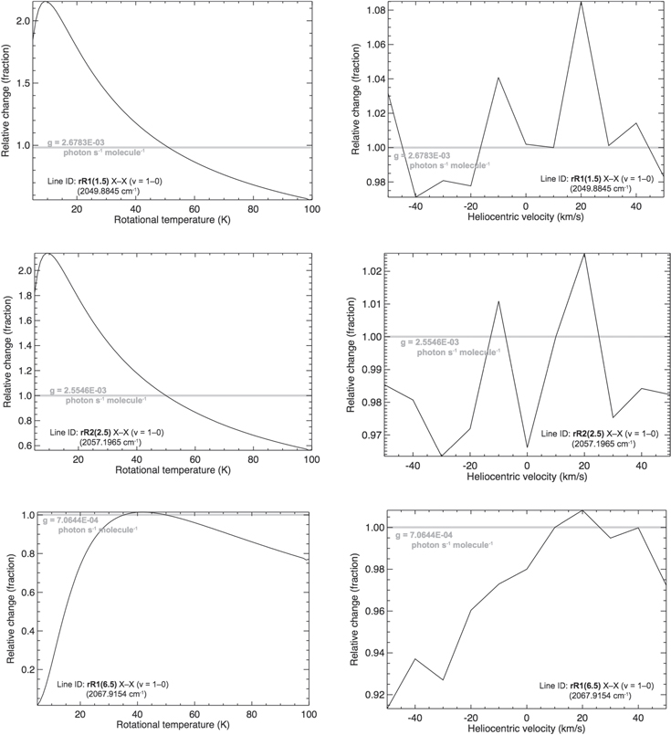
Figure 7. Dependence of fluorescence efficiencies of CN ro-vibrational physical parameters. Left: variation with rotational temperature (considering  km s−1), Right: variation with heliocentric radial velocity (considering Trot = 50 K). These results agree (qualitatively) with studies by Zucconi & Festou (1985) and Schleicher (2010).
Download figure:
Standard image High-resolution image3. IDENTIFICATION OF SPECTRAL LINES FROM ASTRONOMICAL OBSERVATIONS
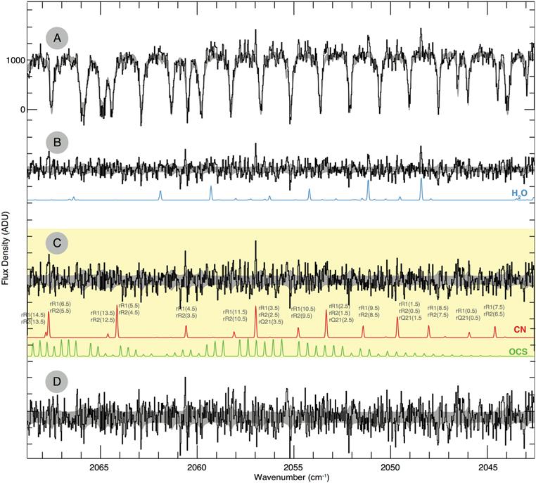
Our observations of comet C/2014 Q2 (Lovejoy) with Keck/NIRSPEC enabled us to sense CN simultaneously with H2O, opening a rather unexplored window to future studies of key volatiles at infrared wavelengths that are complementary to investigations at optical and UV wavelengths. Our model shows a good fit to spectral emission lines of the main CN isotopologue 12C14N in the X2Σ+ system [(1–0) band], measured simultaneously with H2O and OCS (Figure 8). In the observed spectral region, our model predicts R0–R6 (v'−v'') = 1–0) and weak R7–R14 (v'−v'' = 2–1). We are in the process of evaluating the column densities (and production rates) for comparison with other volatiles detected in comet C/2014 Q2. The full results will be presented in a follow-up paper describing our findings (L. Paganini et al. 2016, in preparation).
Figure 8. Comparison of model and observed emission lines in the M-band setting near 4.9 μm using NIRSPEC. Our models predict and match several emission lines from CN (1–0, 2–1), some lines blended with OCS, and strong water lines. (A) Spectrum from the M band showing emission lines, the cometary continuum, and absorption bands due to terrestrial CO2, H2O, and CO. (B) Spectrum with continuum subtracted. (C) The highlighted (in yellow) region shows our CN and OCS models after subtraction of H2O, assuming Trot = 80 K. See Section 3 for further details. (D) Residuals after subtraction of continuum and trace species (H2O, CN, and OCS). Note: spectra in C and D are magnified for clarity. The gray shading represents the 1σ noise.
Download figure:
Standard image High-resolution image
4. SUMMARY
To date, extraction of rotational temperatures, column densities, and production rates from existing high-resolution IR observations of CN has not been possible using high-resolution ro-vibrational lines at IR wavelengths (in the X–X and A–X bands), owing to the lack of fluorescence efficiencies. We have tackled this problem using an RT treatment of the ground vibrational level, and then modeling fluorescence excitation and decay based on Einstein coefficients and line strengths from Brooke et al. (2014), which consider a large number of bands of the A2Π–X2Σ+ and B2Σ+–X2Σ+ systems and ro-vibrational transitions within the X2Σ+ state of CN. Our model includes 40 rotational levels within each of 15 vibrational levels for each (B, A, and X) electronic energy state and accounts for nonresonance fluorescence and the Swings effect. Excitation of the infrared emission lines near 5μm could be pumped by the violet and red systems of CN, whose fluorescence efficiencies are significantly stronger than that by direct infrared vibrational pumping alone. The modeled line-by-line intensities in the (1–0) vibrational band are in good agreement with recent observations of comet C/2014 Q2 (Lovejoy). These fluorescence rates will allow existing and future observations of CN in the NIR, and comparison with simultaneous observations of HCN and other primary nitriles will assist in understanding the role of CN within the taxonomical studies of cometary volatiles.
The authors would like to thank David Schleicher and James S. A. Brooke for interesting insights about this work. We also acknowledge support by NASA's Planetary Astronomy Program (L.P., M.J.M.) and Keck PI Data Award (L.P.), administered by the NASA Exoplanet Science Institute. Data were obtained at the W. M. Keck Observatory from telescope time allocated to the National Aeronautics and Space Administration through the agency's scientific partnership with the California Institute of Technology and the University of California. The authors wish to recognize and acknowledge the very significant cultural role and reverence that the summit of Mauna Kea has always had within the indigenous Hawaiian community.