


Abstract
In this critical compilation, all experimental data on the spectrum of neutral carbon known to us were methodically evaluated and supplemented by parametric calculations with Cowan's codes. The sources of experimental data vary from laboratory to astrophysical objects, and employ different instrumentations, from classical grating and Fourier transform spectrometers to precise laser spectroscopy setups and various other modern techniques. This comprehensive evaluation provides accurate atomic data on energy levels and wavelengths (observed and Ritz) with their estimated uncertainties, as well as a uniform description of the observed line intensities. In total, 412 previously known energy levels were optimized with the help of 1221 selected best-observed lines participating in 1365 transitions in the wavelength region 750 Å–609.14 μm. The list of recommended energy levels is extended by including 21 additional levels found through quantum-defect extrapolations or parametric calculations with Cowan's codes. In addition, 737 possibly observable transitions are predicted. Critically evaluated transition probabilities for 1616 lines are provided, of which 241 are new. With accurate energy levels obtained, combined with additional observed data on high Rydberg states, the ionization limit was determined to be 90820.348(9) cm−1 or 11.2602880(11) eV, in fair agreement with the previously recommended value, but more accurate.
Export citation and abstract BibTeX RIS
1. Introduction
The element carbon, which forms remarkably different allotropes, is essential to life and is the fourth most abundant in the universe. In stars, it takes part in the carbon–nitrogen–oxygen (CNO) cycle and is created via the 3α process. It is ubiquitous in the interstellar medium (ISM) in its numerous forms and plays a major role in the evolution of astrophysical objects (Henning & Schnaiter 1998; Lloyd Evans 2010). Carbon atomic data are vital for (i) solar photospheric determinations of the CNO abundances (Grevesse 1984), (ii) testing the space and time variations of the fundamental constants (Berengut & Flambaum 2010; Curran et al. 2011; Levshakov et al. 2012), and (iii) determination of both astrophysical and chemical conditions of atomic species in various ISM objects (Cardelli et al. 1996; Knapp et al. 2000). More specifically, the isotopic (12C/13C or 14C) spectral line data are important to derive the isotopic evolution of the universe and improve the understanding of nucleosynthesis in stars, to elucidate the effects of isotope shifts in the search for variation of fundamental constants (Berengut & Flambaum 2010; Curran et al. 2011; Levshakov et al. 2012; Murphy & Berengut 2014), and to facilitate laser-based mass spectrometry studies (Clark 1983). In the laboratory, carbon has an extensive usage record, from historic arc-type discharges to various laser-driven plasma sources. It is the most commonly found impurity in laboratory light sources. Carbon data are of high demand in the fusion community (Braams & Chung 2015). Considering the above concerns, consistent and accurate data on wavelengths, intensities, energy levels, ionization energies, and transition rates are always of high priority for a wide range of applications, from the laboratory to astrophysics.
Neutral atomic carbon (C i) contains six electrons arranged as [He]2s22p2 in the ground electronic configuration with five levels, 3P0,1,2, 1D2, and 1S0. The excitation of a single outer electron generates configurations of the type 2s22pnℓ (n > 2, ℓ = s, p, d, f, g, h, ...). Excitation from the closed 2s core produces the 2s2p3 configuration with six terms (5S°, 3D°, 3P°, 3S°, 1D°, and 1P°) and the 2s2p2nℓ (n > 2, ℓ = s, p, d, f, ...) types of configuration. The 2s2p3 configuration is partly above the first ionization limit, and the 2s2p2nℓ configurations are all autoionizing.
Carbon spectral data have been actively investigated since the early 20th century. Many discrete lines of atomic carbon were well known from carbon arc studies (see, e.g., Simeon 1923 and references therein). In early studies, molecular features were dominant in many light sources, obscuring the atomic lines. Merton & Johnson (1923) and Johnson (1925) overcame this hurdle by using a vacuum tube light source (condensed discharge in He) to observe more atomic features of carbon. This method was followed by Fowler & Selwyn (1928) to study the spectrum from the near-infrared (NIR) down to the vacuum ultraviolet (VUV) region. They suggested the wavelength classifications and term values of C i and also interpreted some of the VUV and visible observations of other authors (Bowen & Ingram 1926; Bowen 1927; Ryde 1927). The identifications were extended to a farther infrared (IR) region by Ingram (1929) and to a deeper VUV range by Paschen & Kruger (1930). A few years after, the first composite analysis by Edlén (1934) combined all previous measurements together with his own VUV studies (Edlén 1933a, 1933b) and brought some consistency in the context of the Ritz combination principle. These studies were elaborated by more accurate measurements of the 2p3s–2p3p array in the NIR region (Meggers & Humphreys 1933; Edlén 1936; Kiess 1938; Minnhagen 1954, 1958). Shenstone (1947) established the level value as well as the transition identifications for the  state. Prior to his findings, it was believed impossible to observe transitions from this level in laboratory light sources, because in pure LS coupling they are forbidden.
Carbon lines were proposed as auxiliary wavelength standards in the VUV region (Boyce & Robinson 1936; More & Rieke 1936). To this effect, the most reliable measurements were made by Wilkinson (1955), Herzberg (1958), Wilkinson & Andrew (1963), and Kaufman & Ward (1966). In 1965, Johansson & Litzén (1965) performed Fabry–Perot interferometric measurements of C i in the far-IR region 3868–8604 cm−1 with an uncertainty of ≈0.02 cm−1. Apart from the many LS-allowed and intercombination transitions between the 2p3p and (2p3d + 2p4s + 2s2p3) configurations, they also observed the 2p3d–2p4f transitions. Johansson (1966) made another set of comprehensive measurements using a 21 ft grating spectrograph in the wavelength range 2478–11331 Å and thereby determined more accurate energy levels with uncertainties less than 0.05 cm−1. He observed many new transitions in the 2p3s–2pnp (n = 3–11), 2p3p–2pnℓ (n = 5–10 for ℓ = s; n = 4–11 for ℓ = d), and 2s2p3–2pnℓ (n = 4–8, ℓ = p, f ) arrays. These observations improved upon the accuracy of most of the earlier VUV measurements (Paschen & Kruger 1930; Wilkinson 1955; Wilkinson & Andrew 1963) except those by Herzberg (1958) and Kaufman & Ward (1966).
The next comprehensive compilation of energy levels was carried out by Moore in 1970 (Moore 1970, 1993). Its results were tabulated in her Atomic Energy Levels (AEL) book (Moore 1970), which is hereafter referred to as Moore's table. Her work was largely based on Johansson (1966), but the level values were slightly improved by taking into account several good VUV measurements from Kaufman & Ward (1966), and the intensities of the lines in the VUV region were from photographic examinations (Junkes et al. 1965). Moore's table includes more than 300 Ritz wavelengths of VUV lines, out of which 190 were previously observed. Further VUV line-list enhancements were due to Feldman et al. (1976), who reported Skylab spectra during solar flare activity, and from the flash-pyrolysis photoabsorption spectrum of carbon taken by Mazzoni et al. (1981). In these two studies, extensions of various 2pns and 2pnd  series were made, and more than 50 energy levels were newly established. The high-resolution solar atlas in the 1175–1710 Å region prepared by Sandlin et al. (1986) contains about 192 neutral carbon lines, 46 of which were new, and 103 were more accurate than those from other solar atlases published later (Feldman & Doschek 1991; Curdt et al. 2001; Parenti et al. 2005). Those later atlases also contain some new or improved wavelengths of C i.
Chang & Geller (1998) extended the analysis by combining all available IR data from four different solar spectra (Farmer & Norton 1989; Livingston & Wallace 1991; Toon 1991; Wallace et al. 1993, 1996) together with VUV data of both laboratory (Herzberg 1958; Wilkinson & Andrew 1963; Kaufman & Ward 1966) and solar origin (Feldman et al. 1976; Sandlin et al. 1986). This procedure enabled them to determine the upper energy levels with an average uncertainty of ≈0.014 cm−1. Laboratory improvement of some of these data was carried out by Wallace & Hinkle (2007) via Fourier transform spectra in a wide range of wavelengths from IR to visible. Their method of level optimization and line identifications was limited by their use of Ritz wavenumbers from Chang & Geller (1998), which were correct in most, but not all, cases. Another set of transitions of interest is the parity-forbidden ones within the levels of the 2s22p2 ground configuration. The search for them was initiated in the 1920s (Bowen & Ingram 1926). The 3P1–1S0 transition was subsequently observed for the first time by Boyce (1936) in the spectra of many stellar novae. Several other forbidden lines were also observed in the NIR region in different nebulae (Lambert & Swings 1967; Swensson 1967; Liu et al. 1995). The transitions 3P0–3P1 at 492 GHz and 3P1–3P2 at 809 GHz (see Figure 1) in both stable isotopes 12C and 13C were measured with unprecedented accuracy by several teams (Saykally & Evenson 1980, Cooksy et al. 1986b; Yamamoto & Saito 1991; Klein et al. 1998). These lines of great astrophysical interest are important for studying the astrochemistry of carbon involving the photodestruction of the CO molecule in the ISM (Langer 2009). They were observed in several astrophysical objects (Phillips et al. 1980; Jaffe et al. 1985; Genzel et al. 1988; Frerking et al. 1989; Keene et al. 1998). In 2005, Labazan et al. (2005) measured all three 2s22p2 3P0,1,2  transitions (near 945 Å) with an extremely high accuracy in both stable isotopes. Isotopic shifts were measured for a few more transitions of neutral carbon (Burnett 1950; Holmes 1951; Bernheim & Kittrell 1980). Using an atomic-beam+magnetic-resonance technique, Wolber et al. (1970) measured the hyperfine (HF) level separations and gJ factors of the 12C and 13C 2s22p2 3P term. They also improved the values of the nuclear moment and HF separations of the 3P1,2 states of the unstable 11C isotope (having a lifetime of 20.4 minutes), previously determined by (Haberstroh et al. 1964).
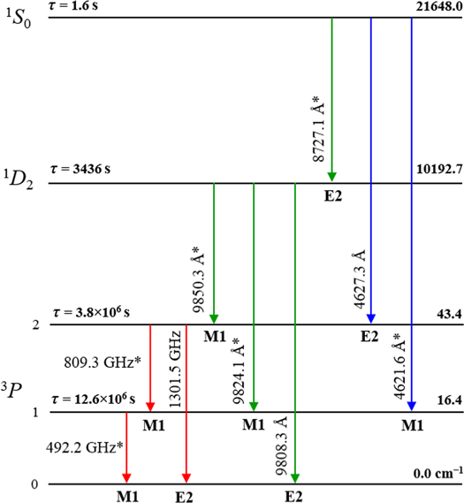
Figure 1. Energy level diagram and forbidden transitions within the levels of the 2s22p2 configuration in C i. Transitions observed in the laboratory and/or astrophysical sources are marked with an asterisk (see Table 3). The lifetime (τ) is derived from A-values compiled by Wiese & Fuhr (2007). The values on the right are level energies in cm−1.
Download figure:
Standard image High-resolution image
C i has received much attention from the theoretical community. Most theoretical studies reporting transition parameters (f- or A-values), Stark shift and broadening parameters, and isotopic shifts, are beyond the scope of the present work. A few exceptions are noted. One of them is a large set of critically evaluated transition rate data (Wiese et al. 1996; Wiese & Fuhr 2007), which has been used and extended in the present work.
The present data on C i in the Atomic Spectra Database (ASD) of the National Institute of Standards and Technology (NIST; see Kramida et al. 2016) are mainly based on the AEL compilation (Moore 1970, 1993). With the growing interest in atomic data, from the perspectives of its various users and numerous applications, the requirements of data reliability and precision are now of the highest priority. In this regard, we note that there exist some disagreements among published fragmented data (Chang & Geller 1998; Wallace & Hinkle 2007). In particular, their stated uncertainties (wavelengths/wavenumbers) were found to be inconsistent with a comprehensive level optimization. Another major problem is related to the relative intensities of transition lines, as they are reported from various measurements made at different experimental conditions. The main aim of the present work is to compile and disseminate a comprehensive and internally consistent set of critically evaluated atomic data on energy levels and observed wavelengths with their uncertainties, as well as uniformly scaled relative line intensities and Ritz wavelengths suitable as secondary standards for the spectrum of neutral carbon.
2. Method of Evaluation of Wavelengths
In neutral carbon, the only VUV transitions observable in emission from non-autoionizing levels are those of the 2s22p2 – [2s2p3 + 2s22pnℓ (n ≥ 3, ℓ = s, d)] arrays, and no other VUV lines occur between the bound states. In such a spectrum, implementation of the Ritz combination principle allows the upper energy levels to be determined with a much greater accuracy than would be possible from measurements only of the VUV transitions. The greater accuracy is achieved by successively measuring each step in the ladder of the 2p3s + 2s2p3 → 2p3p → 2pnℓ (n ≥ 3, ℓ = d, s) transitions, all of which lie above 3279 Å (the ionization threshold from the  state) and summing up the wavenumbers of each step of this ladder and the wavenumbers of the transitions from the first step down to the ground level. The accuracy of levels established in this way is limited by the accuracy of the known transitions between the ground level and 2p3s. As briefly described in the Introduction, the initial implementation of this procedure was made by Johansson (1966), who combined his grating measurements in a wide optical range with the IR Fabry–Perot measurements of Johansson & Litzén (1965). The level accuracy achieved was considered good at the time, but the advent of Fourier transform (FT) spectrometers (FTSs) opened the way for further improvement. Another possibility for improvement appeared after the launch of several missions carrying either high-altitude terrestrial or space-based high-resolution FTSs covering the entire IR solar spectrum, starting in late 1980s (Farmer & Norton 1989; Livingston & Wallace 1991; Toon 1991; Wallace et al. 1993, 1996). Later, the results of these missions were used in the analysis of C i by Chang & Geller (1998). The major problem with solar data was the high level of spectroscopic contamination. This problem was addressed by Wallace & Hinkle (2007), who solved it by replacing the measurements of Chang & Geller (1998) with the measurements of laboratory FTS recordings that were already available in the National Solar Observatory (NSO) archives, but were not analyzed until 2007. The starting point of our investigation was to check the consistency of the measured wavenumbers of Wallace & Hinkle (2007) with their quoted uncertainties using the careful level optimization procedure described by Kramida (2013a). This procedure was successfully implemented in the spectra of many atoms/ions in the past (see, e.g., Kramida 2013b, 2013c; Haris et al. 2014). A satisfactory optimization was achieved by adjusting the initial measurement uncertainties in such a way that the observed wavenumbers agreed with the calculated ones within the adjusted uncertainties. Many new accurate Ritz wavelengths were found in this procedure. These high-precision Ritz-type standards further served as internal references to recalibrate other, less accurate measurements, which were subsequently inserted in the level optimization. On average, the Ritz values are better than most direct measurements by a factor of two or more. Comparison of some sets of measured wavelengths with Ritz-type standards showed noticeable systematic shifts, which needed to be removed before assessing the statistical uncertainties. The entire procedure involved several iterations of level optimization (see Section 3). Consequently, the best available observed wavelengths were kept in the resulting line list reported in Table 1. All optimized observed energy levels for this spectrum are summarized in Table 2.
Table 1. Observed and Predicted Spectral Lines of C i
| Intensitya (arb. u.) | λobsb (Å) | Unc.b (Å) | Lower Levele | Upper Levele | λRitzb (Å) | Unc.b (Å) | A (s−1) | Acc.g | Typeh | TP Referencesi | Line Referencesj | Commentl | ||||
|---|---|---|---|---|---|---|---|---|---|---|---|---|---|---|---|---|
| 1 | 750.680 | 0.010 | 2s22p2 | 3P | 2 | 2s2p2(4P)14p | 3D° | 3 | 750.680 | 0.010 | C81 | GS | ||||
| 1 | 751.240 | 0.010 | 2s22p2 | 3P | 2 | 2s2p2(4P)13p | 3D° | 3 | 751.240 | 0.010 | C81 | GS | ||||
| 1 | 751.420 | 0.010 | 2s22p2 | 3P | 1 | 2s2p2(4P)13p | 3D° | 1 | 751.420 | 0.010 | C81 | GS | ||||
| ... | ... | ... | ... | ... | ... | ... | ... | ... | ... | ... | ... | ... | ... | ... | ... | ... |
| 7800 | 945.18746 | 0.00006 | 2s22p2 | 3P | 0 | 2s2p3 | 3S° | 1 | 945.18745 | 0.00004 | 3.8e+08 | C+ | L89a | L05 | ||
| 17000 | 945.33418 | 0.00006 | 2s22p2 | 3P | 1 | 2s2p3 | 3S° | 1 | 945.33414 | 0.00003 | 1.14e+09 | C+ | L89a | L05 | U | |
| 18000 | 945.57546 | 0.00006 | 2s22p2 | 3P | 2 | 2s2p3 | 3S° | 1 | 945.57546 | 0.00003 | 1.9e+09 | C+ | L89a | L05 | U | |
| ... | ... | ... | ... | ... | ... | ... | ... | ... | ... | ... | ... | ... | ... | ... | ... | ... |
| 730000bl | 1194.028 | 0.014 | 2s22p2 | 3P | 0 | 2s22p5s | 3P° | 1 | 1193.995082 | 0.000020 | 1.94e+07 | A | T01 | M81 | G | |
| 3000000 | 1194.065 | 0.003 | 2s22p2 | 3P | 2 | 2s22p5s | 3P° | 2 | 1194.063006 | 0.000019 | 2.98e+07 | B+ | T01 | S86 | GU | |
| 1100000* | 1194.220 | 0.010 | 2s22p2 | 3P | 1 | 2s22p5s | 3P° | 1 | 1194.229168 | 0.000020 | 8.3e+06 | A | T01 | S86 | G | |
| 1100000* | 1194.300 | 0.010 | 2s22p2 | 3P | 1 | 2s22p4d | 3F° | 2 | 1194.300572 | 0.000019 | 4.1e+06 | B+ | T01 | S86 | G | |
| ... | ... | ... | ... | ... | ... | ... | ... | ... | ... | ... | ... | ... | ... | ... | ... | ... |
| 31000q | 4762.5252 | 0.0005 | 2s22p3s | 3P° | 1 | 2s22p4p | 3P | 2 | 4762.52473 | 0.00006 | 2.7e+05 | C | H93a | W07#2 | FD | |
| 22000q | 4766.6698 | 0.0014 | 2s22p3s | 3P° | 1 | 2s22p4p | 3P | 1 | 4766.66760 | 0.00007 | 2.4e+05 | C | H93a | W07#2 | FC | |
| 24000 | 4770.02392 | 0.00023 | 2s22p3s | 3P° | 1 | 2s22p4p | 3P | 0 | 4770.02376 | 0.00008 | 1.1e+06 | C | H93a | W07#2 | F | |
| 69000 | 4771.73346 | 0.00016 | 2s22p3s | 3P° | 2 | 2s22p4p | 3P | 2 | 4771.73374 | 0.00006 | 8.0e+05 | C | H93a | W07#2 | F | |
| 34000 | 4775.907 | 0.014 | 2s22p3s | 3P° | 2 | 2s22p4p | 3P | 1 | 4775.89266 | 0.00007 | 4.8e+05 | C | H93a | J66 | G | |
| ... | ... | ... | ... | ... | ... | ... | ... | ... | ... | ... | ... | ... | ... | ... | ... | ... |
| 2s22p2 | 3P | 0 | 2s22p2 | 1D | 2 | 9808.295 | 0.003 | 5.9e–08 | C | E2 | F06 | TW | P | |||
| 9824.31 | 0.19 | 2s22p2 | 3P | 1 | 2s22p2 | 1D | 2 | 9824.118 | 0.003 | 7.3e–05 | C+ | M1 | F06 | L95 | GV | |
| 9850.34 | 0.09 | 2s22p2 | 3P | 2 | 2s22p2 | 1D | 2 | 9850.250 | 0.003 | 2.2e–04 | C+ | M1 | F06 | L95 | GV | |
| ... | ... | ... | ... | ... | ... | ... | ... | ... | ... | ... | ... | ... | ... | ... | ... | ... |
| 32000 | 15,727.3506 | 0.0020 | 2s22p3d | 1D° | 2 |
 )4f )4f |
2[3/2] | 2 | 15,727.3529 | 0.0008 | 1.1e+06 | C | H93 | W07#13 | FD | |
| 31000 | 15,784.4994 | 0.0017 | 2s22p3d | 1D° | 2 |
 )4f )4f |
2[5/2] | 2 | 15,784.5012 | 0.0007 | 1.4e+06 | C | H93 | W07#13 | F | |
| 32000 | 15,784.888 | 0.003 | 2s22p3d | 1D° | 2 |
 )4f )4f |
2[5/2] | 3 | 15,784.8896 | 0.0005 | 7.1e+05 | C | H93 | W07#13 | F | |
| 57000q | 15,852.6055 | 0.0018 | 2s22p3d | 1D° | 2 |
 )4f )4f |
2[7/2] | 3 | 15,852.6037 | 0.0005 | 2.1e+06 | C | H93 | W07#13 | FD | |
| ... | ... | ... | ... | ... | ... | ... | ... | ... | ... | ... | ... | ... | ... | ... | ... | ... |
| 2000 | 49,825.54 | 0.025 | 2s22p3d | 3P° | 1 | 2s22p4p | 3P | 1 | 49,825.574 | 0.006 | 1.77e+05 | B | H93a | W07#13* | F | |
| 2600 | 49,934.51 | 0.03 | 2s22p3d | 3P° | 0 | 2s22p4p | 3P | 1 | 49,934.524 | 0.009 | 2.03e+05 | B | H93a | W07#13 | F | |
| 1400 | 50,194.62 | 0.03 | 2s22p3d | 3P° | 1 | 2s22p4p | 3P | 0 | 50,194.627 | 0.008 | 5.7e+05 | B | H93a | W07#13 | FU | |
| ... | ... | ... | ... | ... | ... | ... | ... | ... | ... | ... | ... | ... | ... | ... | ... | ... |
| 6,091,353.36 | 0.24 | 2s22p2 | 3P | 0 | 2s22p2 | 3P | 1 | 6,091,353.37 | 0.24 | 7.93e–08 | A | M1 | F06 | Y91 | V | |
Notes. (A few columns are omitted in this condensed sample, but their footnotes (c, d, f, k) are retained for guidance regarding their form and content.)
aAverage relative observed intensities in arbitrary units are given on a uniform scale corresponding to Boltzmann populations in a plasma with an effective excitation temperature of 0.41 eV, corresponding to the FT spectrum "85R13" (see Section 5 for possible uncertainties in the given values). The intensity value is followed by the line character encoded as follows: bl—blended by other lines either specified by an elemental symbol or given by an index in parentheses. The index is explained as follows (unit of values is cm−1): O iv/2—second order of an O iv line, T—contaminated by a telluric line, 1–23418.059, 2–20992.2792, 3–8254.2325, 4–6834.1017, 5–5657.1101; D—double line; d—diffuse; H—very hazy; i—identification uncertain; m—masked by other lines either marked or specified by an index in parentheses. The index is explained as follows (unit of values is cm−1): 1–21899.0959, 2–2927.0767, 3–2107.4239, 4 = 1350.858, 5 = 1355.422, 6 = 1349.731, 7 = 1347.773, 8 = 1339.013; ℓ–shaded to long wavelength; p—perturbed by nearby lines either indicated by the spectrum symbol or given by an index in parentheses. The index is explained as follows (unit of values is cm−1): gh—grating ghost, 1—8191.0769, 2—8104.4249, 3—6764.1865, 4—6740.0118, 5—5396.8230, 6—3889.1307, 7—2033.1415, 8—2015.0026; q—asymmetric; r—easily reversed; sh—shoulder; w—wide; *—intensity is shared by two or more lines; :—wavelength not measured (the value given is a rounded Ritz wavelength); ?—the given character is uncertain. bObserved and Ritz wavelengths are in vacuum for λ < 2000 Å and λ > 20000 Å and in standard air for 2000 Å < λ < 20000 Å. Conversion between air and vacuum was made with the five-parameter formula from Peck & Reeder (1972). Assigned uncertainty of the given observed wavelength or computed uncertainty of the Ritz wavelength determined in the level optimization procedure. cSignal-to-noise ratio and FWHM (in units of 10−3 cm−1) for the lines measured in FT spectra. dObserved wavenumber (in vacuum) and its uncertainty are given in additional columns in the complete table available in the machine-readable version. eLevel designation from Table 2. fLevel energy value from Table 2. gAccuracy code of the A-value is given in Table 10. hBlank—electric–dipole (E1) transition; M1—magnetic–dipole transition; E2—electric–quadrupole transition. iTransition probability references. All transition probabilities, except those marked as TW ("This work"), are those critically evaluated by Wiese et al. (1996) and Wiese & Fuhr (2007), where the original sources of data were encoded as follows: F06—Froese Fischer et al. (2006); G89a—normalized to a different scale from values reported by Goldbach et al. (1989); H93—Hibbert et al. (1993); H93a—normalized to a different scale from values reported by Hibbert et al. (1993); L89—Luo & Pradhan (1989); L89a—calculated from the multiplet value given by Luo & Pradhan (1989) assuming pure LS coupling; N84—Nussbaumer & Storey (1984); N84a—normalized to a different scale from values reported by Nussbaumer & Storey (1984); T01—Tachiev & Froese Fischer (2001); W—A. W. Weiss, private communication, as quoted in Wiese et al. (1996); and TW—This work, semiempirical calculations using Cowan's codes (see the text). jLine references: B80—Bernheim & Kittrell (1980); C81—Cantù et al. (1981); C98—Chang & Geller's (1998) various solar spectra are designated as #1—NOAO1, Livingston & Wallace (1991), #2—NOAO2, Wallace et al. (1993), #A—ATMOS, Farmer & Norton (1989), #M—Mark-IV, Toon (1991); C01—Curdt et al. (2001); F76—Feldman et al. (1976); F91—Feldman & Doschek (1991); G09—García-Hernández et al. (2009); H58—Herzberg (1958); J66—Johansson (1966); K63—Keenan & Greenstein (1963); K66—Kaufman & Ward (1966); K98—Klein et al. (1998); L95—Liu et al. (1995); M81—Mazzoni et al. (1981); P05—Parenti et al. (2005); R27—Ryde (1927); S47—Shenstone (1947); S86—Sandlin et al. (1986); SiC*—newly observed lines from the SiC FT spectrum; TW—either predicted with accuracy better than that of Johansson (1966) in his Table 3 or newly calculated between energy levels optimized in this work; W07—Wallace & Hinkle (2007), followed by the different origins of the FT spectra from the NSO archive: #1—840210R0.001, #2—810812R0.002, #6—880413R0.006, #13—850905R0.013. See the text in Section 2.1 for more details. An extra "*" denotes either a newly measured line or previous identification revised in this work. See Table 2 for revised energy levels. W63—Wilkinson & Andrew (1963); W96—Wallace et al. (1996); Y91—Yamamoto & Saito (1991). kNumber of sources, if more than one, used to obtain an averaged intensity. lComments: C—uncertainty of the line is the difference between the fitted wavelength and the line's center of gravity; D, E—the given uncertainty was doubled or tripled, respectively, compared to the original value in the quoted source; F—FT measurement; G—grating measurement; P—predicted line; S—single line that solely determines the upper energy level; T—intensity much greater than expected; U—intensity varies by an order of magnitude or more in different observations; V—intensity could not be reduced to the common scale; W—intensity is much weaker than expected; X—the line was excluded from the level optimization; Y—blending reported in the original quoted work is removed in this work.Only a portion of this table is shown here to demonstrate its form and content. A machine-readable version of the full table is available.
Table 2. Observed Energy Levels of C i
| Configurationa | Terma | Ja | Eobs (cm−1) | Unc.(D1)b (cm−1) | Unc.b (cm−1) | Leading Percentagesc | ΔEd (cm−1) | LSa | No.L.e | Commentf | ||||
|---|---|---|---|---|---|---|---|---|---|---|---|---|---|---|
| 2s22p2 | 3P | 0 | 0.0000000 | 0.0000006 | 0.0013 | 98 | −12 | 51 | ||||||
| 2s22p2 | 3P | 1 | 16.4167130 | 0.0000005 | 0.0013 | 98 | −9 | 120 | ||||||
| 2s22p2 | 3P | 2 | 43.4134567 | 0.0000007 | 0.0013 | 98 | −9 | 141 | ||||||
| 2s22p2 | 1D | 2 | 10,192.657 | 0.003 | 98 | 11 | 76 | |||||||
| 2s22p2 | 1S | 0 | 21,648.030 | 0.003 | 94 | 4 | 2p4 1S | 22 | 49 | |||||
| 2s2p3 | 5S° | 2 | 33,735.121 | 0.018 | 100 | 3 | 2 | |||||||
| 2s22p3s | 3P° | 0 | 60,333.4476 | 0.0005 | 96 | −66 | 12 | |||||||
| 2s22p3s | 3P° | 1 | 60,352.6584 | 0.0003 | 96 | −68 | 34 | |||||||
| ... | ... | ... | ... | ... | ... | ... | ... | ... | ... | ... | ... | ... | ... | ... |
| 2s22p3p | 3P | 2 | 71,385.40992 | 0.00006 | 0.00000 | 98 | 23 | 43 | B | |||||
| ... | ... | ... | ... | ... | ... | ... | ... | ... | ... | ... | ... | ... | ... | ... |

|
2[7/2]° | 3 | 86,426.7910 | 0.0006 | 99 | 1 | 4 | |||||||

|
2[7/2]° | 4 | 86,426.7917 | 0.0006 | 99 | 1 | 3 | |||||||

|
2[9/2]° | 5 | 86,427.2556 | 0.0003 | 99 | 1 | 2 | R | ||||||

|
2[9/2]° | 4 | 86,427.25603 | 0.00020 | 0.0004 | 99 | 1 | 2 | R | |||||
| 2s22p5d | 1F° | 3 | 86,449.208 | 0.022 | 92 | 4 | 2p5d3F° | −3 | 4 | |||||
| ... | ... | ... | ... | ... | ... | ... | ... | ... | ... | ... | ... | ... | ... | ... |
 )29d )29d |
2[7/2]° | 3 | 90,753.8 | 0.3 | 1F° | 1 | ||||||||
C ii ( ) ) |
limit | 90,820.348 | 0.009 | |||||||||||
C ii ( ) ) |
limit | 90,883.743 | 0.009 | |||||||||||
| 2s2p2(4P)3s | 5P | 1 | 103,541.69 | 0.24 | 100 | −1 | 1 | |||||||
| 2s2p2(4P)3s | 5P | 2 | 103,562.31 | 0.10 | 100 | 1 | 1 | |||||||
| 2s2p2(4P)3s | 5P | 3 | 103,587.18 | 0.15 | 100 | −2 | 1 | |||||||
| 2s2p3 | 1D° | 2 | 103,762 | 19 | 95 | L | ||||||||
| ... | ... | ... | ... | ... | ... | ... | ... | ... | ... | ... | ... | ... | ... | ... |
| 2s2p2(4P)14p | 3D° | 3 | 133,256.0 | 1.8 | 1 | |||||||||
Notes.
aThe level designations are either in the LS or JK (pair) coupling scheme. JK-designation is given for all previously known regular series 2pnd (n ≥ 7) and 2pnℓ (n ≥ 8, ℓ = s, p), and their old LS designation with a leading percentage is given in the column "LS." bThe quantity given in column "Unc." is the uncertainty of the separation from the "base" level 2s22p3p3P2 at 71,385.40992 cm−1 (see text). The quantity in column "Unc. (D1)" approximately corresponds to the minimum uncertainty of the separation from other levels (for a strict definition, see Kramida (2011). If blank, it is the same as "Unc."). To roughly estimate an uncertainty of any energy interval (except those within the ground term), the values in column "Unc." should be combined in quadrature (see the text in Section 3). cThe first leading percentage refers to the configuration and term given in the first two columns. The second and third percentages refer to the configuration and term subsequent to them. Percentages are blank for levels that were not included in the calculations. dDifferences between Eobs and those calculated in the parametric least-squares fitting (LSF). Blank for unobserved levels or those excluded from the LSF or not included in the calculations. eNumber of observed lines determining the level in the level optimization procedure. Blank for unobserved levels. fB—the base level for presentation of uncertainties; E—the energy level is extrapolated from the known quantum defects; L—the level value obtained in the parametric LSF calculation with Cowan's codes (see text); R—the value of Eobs of previously unresolved fine-structure components is resolved in this work; T—the level position is tentative, based on a single line with an uncertain identification (see Table 1).Only a portion of this table is shown here to demonstrate its form and content. A machine-readable version of the full table is available.
Download table as: DataTypeset image
2.1. Measurements of Wallace and Hinkle
As briefly mentioned above, the reported wavenumbers of Wallace & Hinkle (2007) originate from three (out of four) spectrograms archived at the Virtual Solar Observatory (VSO) repository of the Kitt Peak National Observatory (KPNO), Tucson, AZ, where a 1 m (f/55 IR-visible-UV) FTS facility works in conjunction with either the McMath telescope's main beam or with laboratory sources (Brault 1978). We obtained all those spectrograms from VSO (Hill et al. 2004), archived as 1981/08/12R0.002, 1984/02/10R0.001, 1985/09/05R0.013, and 1988/04/13R0.006 (hereafter called 81R02, 84R01, 85R13, and 88R06, respectively), and remeasured them, as it was necessitated by the lack of detailed data on the wavenumber measurement uncertainties in Wallace & Hinkle (2007). Those authors gave estimates of the systematic correction factors (with their uncertainty) for FTS-measured wavenumbers, and their table contains corrected wavenumbers and relative intensities. However, to determine the statistical uncertainties, we also need to know the line width and signal-to-noise ratio (S/N) for each line, which were not included by Wallace and Hinkle. Their paper also lacks any indication of the possible blending or distortions of the observed line profiles. We tried to use the limited general information about the line widths given by Wallace and Hinkle to derive estimates of statistical uncertainties, but all these attempts led to a large inconsistency between the observed and Ritz wavenumbers for many lines. Thus, we repeated the reduction of all available FTS recordings, including the calibration, determination of the S/N ratio, and careful characterization of each line profile.
Among the four spectrograms, 85R13 contains the largest number of carbon lines (more than 270). It was taken by P. F. Bernath, using a microwave (μ) discharge in a helium/methane mixture (367/4 Pa or 2.75/0.03 Torr) with the addition of phosphorous, at a resolution of 0.02 cm−1 in the 1630–9860 cm−1 region. The high-resolution (≈0.01 cm−1) spectrogram 84R01, taken by J. W. Brault with a C/Ne/CO (430/20 Pa or 3.2/0.15 Torr) hollow cathode lamp, covers the spectral region 1418–9406 cm−1 and has a significant number of carbon lines, but its signal strength is low compared to the μ-discharge spectrum. Further down to the red end of the spectrum, the region 8995–16,010 cm−1 is covered by the spectrogram 88R06 recorded by P. F. Bernath with a helium/allene (190/13 Pa or 1.4/0.1 Torr) μ-discharge at a resolution of 0.02 cm−1. It contains about 20 lines of C i. The last spectrogram, 81R02, was acquired by J. W. Allen with an electrodeless discharge in a Ne/CH4 (150/1.7 Pa or 1.1/0.013 Torr) mixture at a 0.03 cm−1 resolution. It covers the optical region 15,477–27,000 cm−1, but it has only 15 C i lines.
The wavenumbers, S/Ns, line widths, and intensities were determined from the FTS spectrograms with the help of the DECOMP program (Brault & Abrams 1989) implemented for the X-windows graphical environment of Unix-based operating systems in the code XGREMLIN (Nave et al. 2015), which can find a least-squares fit to the Voigt profile of each line. In FT spectra, the scale of the measured wavenumbers (σmeas) must be corrected. Although a well-controlled He–Ne sampling laser produces a fairly linear wavenumber scale, there remains some degree of imperfection in the alignment of the optical beams from the laser and the light source, along with effects due to the finite entrance aperture size. In this regard, a multiplicative correction factor is derived from a set of accurately known reference wavenumbers (σref), either of buffer-gas atomic lines or of molecular features present in the spectrum. The corrected wavenumber (σcor) can be expressed as

where keff is a weighted mean of individual correction factors from each reference line,  , with weight wi equal to the inverse square of the total uncertainty δki. The latter is a combination in quadrature of the relative statistical uncertainty in σmeas and the relative uncertainty in σref. The uncertainty in keff is estimated by the expression

given by Radziemski & Andrew (1965). We note that Equation (2) is similar to the equation defining the uncertainty D1 in the level optimization code LOPT (Kramida 2011) and is an empirical extension of the standard statistical expression for the uncertainty of a weighted mean,  . This extension empirically accounts for various irregular systematic effects, such as line blending, which are often present in spectroscopic measurements.
The global systematic uncertainty in wavenumbers is estimated as δσsys = σ × δkeff. The statistical uncertainty can be obtained from the formula given by Davis et al. (2001),

where kg is a scaling factor depending on the choice of the fitting function (close to 1.0), W is the full line width at half maximum (FWHM), and NW is the number of statistically independent data points in FWHM, defined as the ratio of the measured FWHM to the instrumental resolution. The final total uncertainty of a measured wavenumber is the sum in quadrature of the statistical uncertainty and the global systematic uncertainty (Redman et al. 2014).
The infrared spectrogram 85R13 is underresolved (i.e., NW < 4) and contains many atomic and molecular lines (mainly due to hydrogen, helium, oxygen, phosphorous, argon, and carbon monoxide) and additional noisy features of instrumental origin. The measurements were made after the background subtraction and interpolation of the spectrum, which doubled the number of data points in it. The calibration was made with recommended infrared standards of the 1–0 band of carbon monoxide (Maki & Wells 1992), and the systemic correction factor (obtained using 12 well-resolved reference lines) is keff = 5.60(18) × 10−7, which is about the same as that reported by Wallace & Hinkle (2007; 5.8 × 10⁻⁷). However, their systematic uncertainty was a factor of 3/2 greater than ours, as they used less accurate wavenumbers from Guelachvili & Narahari Rao (1986).
For the supplementary IR spectrogram 84R01, we obtained keff = 5.5(3) × 10−7 using 23 low-excitation (3p → 4s) reference lines of Ne i (Saloman & Sansonetti 2004) that have relative uncertainties of 9 to 12 parts in 108. We note that the CO lines had irregular shapes in 84R01 and were unsuitable for calibration. We also used some C i lines that appeared in both the 84R01 and 85R13 spectrograms to derive the calibration constant for 84R01, which turned out to be the same as that from the Ne I calibration. For both the 84R01 and 85R13 spectrograms, we take kg = 1.5, since the number of data points in the observed line width was small, NW ≈ (1.5–3). We deduced this value of kg from numerical simulations.
Five low-excitation (4s → 4p) Ar i lines (Sansonetti 2007) served as internal standards to calibrate the 88R06 spectrum in the 8995–16,010 cm−1 region, resulting in keff = −3(6) × 10−8. Even though Wallace & Hinkle (2007) used the Ar I wavenumbers from Whaling et al. (2002) affected by an error in the systematic correction found later by Sansonetti (2007), our value essentially agrees with theirs, +5(9) × 10−8.
The spectrogram 81R02 covering the region 15,477–27,000 cm−1 was calibrated with seven strong 4s → 5p lines of Ar I (Sansonetti 2007). A value keff = −5.7(3) × 10−7 was determined in agreement with that of Wallace & Hinkle (2007), −5.3(3) × 10−7. In addition to Ar i, this spectrum contains many strong Ne I lines. However, most of them are from higher excited levels (4d, 5d, 6s, 7s, 8s) and produce a different value of keff (30% smaller). This may be explained by a different spatial origin of these lines, and/or by isotope shifts (which are larger in Ne than in Ar), and/or by possible Stark shifts, which are stronger for higher excited levels. Therefore, these high-excitation Ne lines were not included in the calibration.
The corrected wavenumbers with their assessed uncertainties and assignments were then taken into a preliminary level optimization process. As mentioned above, since the spectrum 85R13 is underresolved, the lines are affected by ringing or side lobes of strong nearby features, blending by known or unidentified lines, and asymmetries in the line shape. Those affected lines were double-checked (see Section 3) at various stages of the level optimization process.
2.2. Observations of Johansson & Litzén and Johansson
The measurements of Johansson & Litzén (1965) and Johansson (1966), made with a Fabry–Perot interferometer and a grating spectrograph, respectively, are an extensive source of atomic data for C i. The FT spectrogram 85R13 fully superseded the IR measurements of Johansson & Litzén (1965), whose estimate of uncertainty was better than 0.02 cm−1. We re-assessed the uncertainty with the aid of Ritz wavenumbers from the FT spectra. It turned out that most of the wavenumbers reported by Johansson and Litzén agree with the Ritz ones with a standard deviation (hereafter, uncertainty) of 0.01 cm−1, except for the unresolved features.
The other set of measurements of Johansson (1966) was made with two different grating spectrographs. For wavelengths λ < 9600 Å, he used a 21 ft concave grating spectrograph with a reciprocal linear dispersion (hereafter, dispersion) of 5 Å mm–1 in the first order of diffraction. Wavelengths below 4700 Å were measured in the second order of this instrument. For the wavelengths in the range 10,000–11,600 Å, a plane grating spectrograph was used in the second order, where it had a dispersion of ≈2 Å mm–1. Johansson reported wavelengths of 380 C i lines in the 2478–11,331 Å range, most of which were given with three digits after the decimal point. From the FTS spectra described in the previous section, augmented with accurately measured VUV lines (see Section 2.4), we selected 104 uniquely classified and well-resolved lines having Ritz wavelength uncertainties in the range 0.00006–0.0018 Å to examine the wavelengths reported by Johansson in the three spectral regions described above. A comparison of the observed and Ritz wavelengths yielded our estimated uncertainties for Johansson's measurements: 0.005 Å, 0.014 Å, and 0.009 Å for λ < 4700 Å, 4700–9600 Å, and λ > 9600 Å, respectively; no significant systematic errors were found. These values are about a factor of two smaller than Johansson's estimates of the upper bounds of the uncertainties.
2.3. Observations of Transitions within the Ground Configuration
Forbidden transitions (M1 and E2) between the levels of the ground configuration 2s22p2 are distributed in three regions, far-infrared (FIR), NIR, and optical, as can be easily inferred from Figure 1. As mentioned above, some of these NIR and/or optical transitions were observed in several astrophysical objects (Boyce 1936; Lambert & Swings 1967; Swensson 1967; Liu et al. 1995). The implementation of the FIR-laser magnetic-resonance (FIR-LMR) technique (Saykally & Evenson 1980) brought about the first precise laboratory values for the 3P0–3P1 and 3P1–3P2 transitions at ≈492 and ≈809 GHz, respectively, for both 12C and 13C isotopes. We accepted the most precise and accurate measurements available now for the 3P0–3P1 (Yamamoto & Saito 1991) and 3P1–3P2 (Klein et al. 1998) transitions. Yamamoto & Saito (1991) used a source-modulation microwave spectrometer together with a 2 m long free space cell, while a Cologne terahertz spectrometer detection system was used by Klein et al. (1998). Both these experiments produced carbon atoms by a discharge in CO+He mixtures (kept at very low pressures ≈5 Pa or 38 mTorr) at liquid nitrogen temperature. The reported uncertainties of these measurements were given on the level of two or three standard deviations, and we reduced them to the 1σ level to provide a uniform representation of uncertainties in all data (see Table 3).
Table 3. Observed Astrophysically Important Forbidden Transitions of C i (12C/13C) from Laboratory and Astrophysical Sources
| Transition | Species | Laboratory a | Astronomical b | Ritz c | A (s−1) d | References e | |
|---|---|---|---|---|---|---|---|
| 12C | 492,160.651(18) | 492,160.651(18) | Y91 | ||||
| 3P0–3P1 | 13C | 492,162.900(35) | 492,162.889(18) | 7.93e−08 | A | Y91 | |
| C | 492,160.675(19) | 492,160.7(1) | 492,160.675(18) | Y91, F89 | |||
| 12C | 809,341.970(17) | 809,342.3(4) | 809,341.970(17) | K98, K98a | |||
| 3P1–3P2 | 13C | 809,346.1(1) | 809,346.103(44) | 2.65e−07 | A | K98 | |
| C | 809,342.01(2) | 809,342.014(17) | K98 | ||||
| 12C | 1,301,502.621(25) | ||||||
| 3P0–3P2 | 13C | ... | ... | 1,301,508.990(48) | 1.72e−14 | B+ | ... |
| C | 1,301,502.689(25) | ||||||
| 3P2–1D2 | C | ... | 9850.34(9) | 9850.250(3) | 2.2e−04 | C+ | L95 |
| 3P1–1D2 | C | ... | 9824.31(19) | 9824.118(3) | 7.3e−05 | C+ | L95 |
| 3P0–1D2 | C | ... | ... | 9808.295(3) | 5.9e−08 | C | ... |
| 1D2–1S0 | C | ... | 8727.126(8) | 8727.131(3) | 6.0e−01 | B | W96 |
| 3P2–1S0 | C | 4627.3438(22)f | ... | 4627.3444(6) | 2.2e−05 | C | TW |
| 3P1–1S0 | C | 4621.5695(7) | 4261.4 | 4621.5693(6) | 2.3e−03 | C+ | TW, B36 |
Notes.
aFor all transitions, except the first three, the observed and Ritz wavelengths (in standard air) are given in Å. For the first three transitions, the observed and Ritz frequencies in units of MHz are given in italics. Multiple values given in consecutive rows are for 12C, 13C, and natural C; a single value represents natural C samples; the value in parentheses is the 1σ uncertainty in the last significant digit. bThe best available astronomical data; the uncertainties are from the original measurements. cThe Ritz values from the level optimization made in this work (see Sections 3 and 4). dThe transition rates (A-values) with the stated accuracy in the next column are from Wiese & Fuhr (2007). The accuracy code is described in Table 10. eReference code for the values in columns 2 and 3, respectively: B36—Boyce (1936); F89—Frerking et al. (1989); K98—Klein et al. (1998); K98a—Keene et al. (1998); L95—Liu et al. (1995); TW—this work, from the 81R02 FT spectrum; Y91—Yamamoto & Saito (1991); W96—Wallace et al. (1996). fThe identification is questionable.Download table as: ASCIITypeset image
One of the accurately measured transitions is (2s22p2)3P1–1S0 at 4621.5695(7) Å, observed with S/N = 17 on the 81R02 FT spectrogram. This spectrogram was acquired with the lowest buffer-gas pressure among all other FT spectra described above (see Section 2.1). To validate an observation of a forbidden transition in such a laboratory spectrum, many considerations were taken into account. From the analysis of observed C i line intensities, it was found that the effective excitation temperature ( ) in this spectrum was 0.28 eV, which is the lowest among the FT spectra analyzed here. The low lamp pressure and temperature imply that the electron density was minimal, which favors the observation of this forbidden transition. In this regard, we note that it requires about twice as much energy to ionize neon atoms than carbon atoms. The
  derived from the lines of Ne I was 0.20 eV. The validity of both derived source temperatures was verified by comparing the wavelength-dependent instrument-response functions derived from the C i and Ne i spectra, which agreed with each other (see Kramida 2013a, 2013b, 2013c; Haris et al. 2014 for technical details of the methods used in this derivation). Under such low temperatures, most of the free electrons in the plasma originate from singly ionized carbon atoms. Under LTE conditions, the fraction of
  in the discharge would be about 1% (see the Saha–Boltzmann plot for a C+N mixture in the NIST ASD; Kramida et al. 2016), which should result in electron densities ne < 1014 cm−3. This estimate is supported by a rough determination of ne from the measured Stark width ws of the hydrogen
  line at λ = 4861.323 Å (hydrogen was present as a small impurity in the spectra we analyzed). From the measured value of ws ≈ 0.06 Å, we derived the value of ne of the order of 1013 cm−3. The plausibility of an observation of forbidden lines within the ground configuration of C i under these conditions is indirectly supported by findings of Eriksson (1965), who observed a similar forbidden transition within the ground configuration of O i with an electrodeless discharge lamp that had a similarly low pressure.
We searched for the two transitions from the same upper level and found a faint asymmetric line (with S/N just above 3) at 4627.3438(22) Å corresponding to the 3P2–1S0 transition, which we adopted as a questionable identification, since our predicted intensity of this transition is two orders of magnitude lower than observed. We investigated all impurities present in the 81R02 spectrum and did not find any known line belonging to these impurities that could mask or blend with this line. No other forbidden lines were observed in the visible range, except the line at 8727.126(8) Å (1D2–1S0) reported by Wallace et al. (1996) from solar observations. Among the NIR transitions, the 3P1–1D2 and 3P2–1D2 lines were observed in several astrophysical objects (Swensson 1967; Liu et al. 1995), and their averaged observed wavelengths are 9824.31(19) and 9850.34(9) Å, respectively. All these observations are summarized in Table 3 together with critically evaluated theoretical transition rates (Wiese & Fuhr 2007) and accurate Ritz values derived in this work.
2.4. Vacuum Ultraviolet FTS Measurements
Griesmann & Kling (2000) made accurate interferometric measurements of lines of carbon and other elements in the VUV range. They kindly permitted us to use their unpublished data obtained during that work, in which we found 14 lines of C i. Their measurements were made with the FT700 VUV FT spectrometer at NIST (Griesmann et al. 1999) using a Penning discharge with silicon carbide (SiC) cathodes and Ne as carrier gas with a small addition of Ar. The unpublished data of Griesmann and Kling included recordings of two interferograms containing features of neutral carbon. One of these recordings, covering the spectral region of 14,883 to 60,350 cm−1 at a resolution R = 0.05 cm−1, had a calibration factor of 7.16(12) × 10−7, as determined by Griesmann and Kling using Ar ii lines (Whaling et al. 1995). It contained only two C i lines corresponding to transitions from  terminating on 1S0 and 1D2 of 2s22p2.
The second spectrum with R = 0.25 cm−1, covering the range 52,000–78,000 cm−1, also provided by Griesmann and Kling, was most useful for our purpose. It contained 11 accurately measured VUV lines of the 2s22p2 3P–(2p3s 3P° + 2s2p3 3D°) transitions, as well as of 2s22p2 1D2– . For this spectrogram, we derived the calibration factor of 1.95(6) × 10−6 from the two Si ii lines measured by Griesmann & Kling (2000). Statistical uncertainties of measurements of this spectrogram are in the range 0.0006–0.017 cm−1. However, as follows from the uncertainty in the calibration factor, there is a relatively large systematic component (≈0.004 cm−1 or 0.00010 Å) in the total uncertainty of the C i lines in the range of this spectrum. The best earlier measurements for these VUV lines were made with grating spectroscopy by Kaufman & Ward (1966). By comparing their reported wavelength with our FTS measurements and with the Ritz wavelength, we found that the measurements of Kaufman and Ward had a small systematic shift of about −0.0006 Å, which we removed from their reported wavelengths. After that, the remaining statistical uncertainty of a few lines adopted from Kaufman and Ward is estimated to be 0.0008 Å.
2.5. Observations of Chang and Geller
The C i lines reported by Chang & Geller (1998) originated from four sets of FTS measurements of solar spectra. Some of them were space-based, some balloon-borne, and some ground-based. The largest number of lines, 148, is from the space-based ATMOS mission and covers the 600–4800 cm−1 region (Farmer & Norton 1989). About 40 C i lines are from the balloon-borne MARK IV observation (Toon 1991). Both these spectra are reasonably free from telluric contamination. The other two observations are from the McMath telescope in conjunction with the 1 m FTS of KPNO, in the regions of 1850–9000 cm−1 (Livingston & Wallace 1991, hereafter NOAO1) and 8900–13,600 cm−1 (Wallace et al. 1993, hereafter NOAO2). Most of these measurements were superseded by laboratory FTS measurements. However, extraordinary conditions could exist in the solar atmosphere, making it possible to observe some transitions that could not be observed in laboratory light sources. Indeed, we found such transitions in these solar spectra.
None of the original solar line lists mentioned above explicitly reported the measurement uncertainties. However, notes in Chang & Geller (1998) on possible blending and other factors affecting the measurements were helpful in our assessment of uncertainties, which was mainly based on comparisons with the Ritz wavenumbers derived from laboratory spectra. The statistical uncertainty was estimated using Equation (3), under the assumption that the weakest observed lines had S/N = 1, and that the line widths were largely due to Doppler broadening. The latter was estimated using the photospheric temperature Tphot = 5500 K, which is consistent with the Boltzmann plots used in the intensity reduction (see Section 5). Many wavelengths were still deviating too much from the Ritz values, which forced us to increase the statistical uncertainty of many perturbed lines (blended, appearing on shoulders of stronger lines, or contaminated by telluric features) to half of their width irrespective of their intensity. The unweighted systematic correction factors and their uncertainties were estimated using accurately known C i Ritz wavenumbers. Corrections to the originally reported calibration were found to be much smaller than statistical uncertainties; hence, all originally reported wavenumbers were retained in this work. For the ATMOS spectrum, by using 19 Ritz standards, we obtained a global systematic correction keff = 7(6) × 10−7 to the wavenumbers listed by Chang and Geller. Statistical uncertainties of lines from this spectrum are in the ranges 0.006–0.015 cm−1 and 0.006–0.022 cm−1 for unperturbed and perturbed lines, respectively. The MARK IV spectrum was compared with 13 Ritz wavenumbers accurate to better than 0.008 cm−1; keff = 6.6(19) × 10−7 was derived. For this spectrum, statistical uncertainties were in the range 0.007–0.026 cm−1. The ground-based observations are more prone to atmospheric contamination. The correction factors and statistical uncertainties were found to be keff = −5.3(20) × 10−7, δσstat = 0.0004–0.040 cm−1, and keff = +5.1(25) × 10−7, δσstat = 0.0003–0.062 cm−1 for NOAO1 and NOAO2, respectively. After combining both systematic and statistical uncertainties in quadrature, 74 lines from these four spectra were added to the C i line list. All these lines correspond to electric–dipole (E1) transitions. Some of them are intercombination (spin-changing) transitions, some involve a change in total angular momentum ΔL > 1 or in the orbital angular momentum of the outer electron Δℓ > 1 (enabled by weak mixing between different configurations), and the rest are from highly excited levels (5f−6g and 5g–6h transitions). All of these types of transitions are difficult to observe in laboratory conditions.
It is important to mention here that the ATMOS measurements were followed by similar solar measurements with the Atmospheric Chemistry Experiment (ACE) FTS on board the Canadian SCISAT-1 satellite (Hase et al. 2010). The measurement accuracy of ACE-FTS was inferior to that of ATMOS because of the twice lower resolution. Nonetheless, the accuracy of the observed line intensities was much improved by co-adding multiple recordings. Thus, the ACE-FTS data were used for intensity reduction (see Section 5).
2.6. Observations of VUV Transition Arrays
VUV transition arrays of C i were observed in many laboratory sources (Fowler & Selwyn 1928; Paschen & Kruger 1930; Edlén 1933b; Wilkinson 1955; Herzberg 1958; Wilkinson & Andrew 1963; Kaufman & Ward 1966; Junkes et al. 1965; Mazzoni et al. 1981), as well as in several solar prominences (Feldman et al. 1976; Sandlin et al. 1986; Feldman & Doschek 1991; Curdt et al. 2001; Parenti et al. 2005). These measurements were compared with Ritz wavelengths (accurate to better than 0.0003 Å) generated using long-wavelength FTS measurements in combination with several VUV lines precisely measured with an FTS (see Sections 2.1–2.5). Evaluated uncertainties of individual measurements with a brief description of observations are tabulated in Table 4. No significant systematic shifts were found in these measurements.
Table 4. List of Vacuum Ultraviolet Measurements in C i with Their Evaluated Uncertainties
| Sourcea | No. of linesb | Range (Å) | Unc.c(mÅ) | Descriptiond | δλ/δxe(Å mm–1) |
|---|---|---|---|---|---|
| F28 | 15 | 1260–1752 | 60 | CO2–He; G; Ph | 10 |
| P30 | 94 | 1112–1400 | 50 | He–C HC; 1 m G; Ph | 8.5 |
| 21 | 1400–2950 | 50 | 17.5 | ||
| E33b | 15 | 945–1659 | 20{≈10} | Vacuum spark; 1 m G; Ph | 8.3 |
| B36 | 100 | 945–1994 | 30 | Gas discharge; 2 m G; Ph | 4.3 |
| S47 | 9 | 1430–1660 | 10{10} | Carbon arc; 21 ft G; Ph | 1.3 |
| 3 | 2582–2968 | 2{2} | Carbon arc; Q; Ph | ||
| W55 | 43 | 1158–1931 | 5{5} | HC; 21 ft G; Ph | 1.3 |
| H58 | 6 | 1328–1330 | 0.7{0.7} | HC; 3 m G; Ph | 0.6[5] |
| W63 | 14 | 1560–2478 | 3{1} | HC; 21 ft G; Ph | 0.4[3] |
| J65f | 180 | 1116–2252 | ⋯ | HC; 1 m G; Ph | 8.1 |
| K66g | 18 | 1459–1931 | 0.8{1} | HC; 10.7 m G; Ph | 0.78 |
| F76 | 120 | 1100–1930 | 10; 4{10; 4} | Solar flare; 2 m G; Ph | 4.2[2] |
| C81 | 33 | 750–870 | 10{10} | AFP; 2 m G; Ph | 4.2 |
| M81 | 150 | 1100–1161 | 10; 5{10} | AFP; 2 m G; Ph | 4.2 |
| <1200 | 7{10} | ||||
| S86 | 200 | 1188–1660 | 10; 3{10; 3} | SP; 2 m G; Ph | 4.2[2] |
| F91 | 45 | 1114–1160 | 10{10} | ||
| C01 | 216 | 945–1610 | 10{10} | SP; 3.2 m G; MCP | 0.87 |
| P05 | 100 | 945–1260 | 20–40h | ||
| L05 | 3 | ≈945 | 0.06i | C2H2/He; tunable XUV laser | ⋯ |
Notes.
aSource reference code: B36—Boyce & Robinson (1936); C81—Cantù et al. (1981); C01—Curdt et al. (2001); E33b—Edlén (1933b); F28—Fowler & Selwyn (1928); F76—Feldman et al. (1976); F91—Feldman & Doschek (1991); H58—Herzberg (1958); J65—Junkes et al. (1965); K66—Kaufman & Ward (1966); L05—Labazan et al. (2005); M81—Mazzoni et al. (1981); P30—Paschen & Kruger (1930); P05—Parenti et al. (2005); S47—Shenstone (1947); S86—Sandlin et al. (1986); W55—Wilkinson (1955); W63—Wilkinson & Andrew (1963). bTotal number of observed lines in each source. cUncertainties evaluated by comparing the observed and Ritz wavelengths of unperturbed lines (see text in Section 2.6), and/or the originally reported values in curly brackets. When two figures separated by a semicolon are given, they correspond to wavelengths reported with two and three decimals after the point, respectively. For perturbed lines (e.g., blended, doubly classified, or shaded), the given uncertainty is doubled. dA brief experimental description of the light source, instrument, and detector used. The symbols HC, G, Ph, Q, AFP, SP, and MCP denote hollow cathode discharge, grating, photographic plate/film, quartz prism, absorption with flash pyrolysis, solar prominences, and microchannel plate, respectively. eInverse linear dispersion (in the first order of diffraction unless the order is specified in square brackets). fOnly intensities were measured, but not wavelengths. gA systematic shift of −0.0006 Å was removed from the originally reported values (see Section 2.4). hThe given value is quoted from the original work. Our comparison shows an average uncertainty of 30 mÅ. iUncertainty could not be estimated in this work as the upper level of all transitions from this source relies entirely on the observations therein; the original value is quoted.
Download table as: ASCIITypeset image
2.7. Observations of Other Transitions
The spin-forbidden (intercombination) 2s22p2 3P1,2– transitions near 2966 Å were first measured by Shenstone (1947) with an uncertainty of 0.002 Å and later remeasured for the 12C and 13C isotopes by Bernheim & Kittrell (1980) in the 19th order of a grating spectrometer. Once the most accurate measured wavelengths were selected for each firmly identified transition and their uncertainties were evaluated, we reoptimized the energy levels and searched for possible identification of previously unclassified lines in published line lists. We found many suspected C i lines in the list of lines observed by Keenan & Greenstein (1963) in a spectrum of a carbon-rich star R Coronae Borealis (R-CrB). About 240 C i lines were already identified by those authors based on laboratory observations (Johansson 1966), but a possible extension of the 2p3s → np and 2p3p → (ns + nd) series could be expected due to the peculiarity of stellar conditions, where low densities allow high excitations to be observed. The measurements of Keenan & Greenstein (1963) were primarily divided into two sections, below λ = 4900 Å and above that. Our estimated uncertainties are 0.10 Å and 0.20 Å (for unperturbed and perturbed lines, respectively) for the short wavelengths and 0.16/0.28 Å, respectively, for the longer wavelengths. The above uncertainties are twice the standard deviations (SD) of the observed wavelengths from our Ritz values, allowing for possible unreported blending in this spectrum, strongly contaminated with lines of many chemical elements and molecules. Accordingly, we utilized 51 lines, mostly belonging to the 2p3p → (ns + nd) transition arrays, from Keenan & Greenstein (1963) in the level optimization procedure.
2.8. Autoionizing States
Data on autoionizing states of carbon are important for studies of radiation transport in stars. The ionization continuum of C i essentially starts from the first series limit, C ii  at 90,820.348 cm−1 (see Section 7). Among the regular configurations involving excitation of one 2p electron, only high Rydberg states of 2s22pnℓ converging to the second limit (C ii
  at 90,883.743 cm−1) are autoionizing. All other excited configurations, 2s2p2nℓ, 2p3nℓ, 2p4, and those involving excitation from the inner 1s shell lie above the ionization threshold, except 2s2p3, in which the 5S°, 3D°, and 3P° levels are bound, but 3S°, 1D°, and 1P° are above the ionization limit.
Not all states above the first limit easily decay by autoionization. For some of them, autoionization is strongly forbidden by selection rules (for example, quintet states), and some have competing rates for autoionization and radiative decay. The first observation of such radiative transitions was made for the decay of  to the ground 3P term near 945 Å by Edlén (1933b). The wavelengths of these transitions are now known with an accuracy of 6 parts in 108 (Labazan et al. 2005). In pure LS coupling, the
  state would be strictly forbidden to autoionize. In fact, autoionization is possible due to a minute admixture of the 3P° and 1P° character in its eigenvector composition (0.00013% and 0.0005%, respectively, per our LSF described in Section 6). The total radiative decay rate of 3.41 × 10⁹ s−1 is comparable to the autoionization rate of 1.50 × 10⁹ s−1 (Wang et al. 2013). The autoionization of
  is responsible for about 30% of its total decay rate and significantly contributes to the observed widths of radiative transitions, ≈1 GHz (Labazan et al. 2005). The smallness of the autoionization rate of this state enables the observation of other radiative transitions terminating on 2p3p 3P, which Johansson (1966) identified near 2903 Å in the spectrum of a high-current arc observed by Ryde (1927). The observations by Goly (1976), who measured the radiative rates of these lines, further substantiated the above identification.
Transitions from the quintet term 2s2p23s 5P to  were found by Shenstone (1947) near 1432 Å, which helped him to identify two observed lines near 2966 Å as intercombination transitions between 2s22p2 3P1,2 and
  , and hence to locate the latter level precisely. Edlén (1947) confirmed this identification by an isoelectronic comparison.
Thirty-three strong absorption features due to the 2s22p2 3P–2s2p2np 3D° (n = 3 to 14) transitions were observed by Cantù et al. (1981) in the photoionization spectrum between 750 Å and 870 Å. Of those, the  and
and  series were the most extensive. The 2s2p2np 3D° series converge to the C ii 2s2p2 4P limits at about 43,003 cm−1 above the ground state of C ii,
  , while the C ii
  level has an excitation energy of only ≈63 cm−1. Therefore, the final state of autoionization decay of the C i 2s2p2np 3D° levels can be either of these two C ii levels. Due to constraints on excitation conditions, most laboratory photoionization data on C i are for excitation from the ground 3P term to continuum states. However, contributions of excitation from 1D and 1S (of 2s22p2) to, for example, 2s2p3 1D° and 1P° embedded in the continuum can be significant in astrophysical objects. Complexities in producing a high-temperature vapor of neutral carbon explain the scarcity of experimental photoabsorption studies, of which Hofmann & Weissler (1971) and Marrone & Wurster (1971) are rare exceptions. So far, no experimental data on the exact position of the strongly autoionizing 2s2p3 1D° and 1P° states have been obtained, either by optical or electron spectroscopy. The AEL (Moore 1970) gives their respective energy positions at 97,878 cm−1 and 119,878 cm−1. These values were derived by Edlén (1933b) from an isoelectronic extrapolation. We used the parametric least-squares fits (see Section 6) to pin down their positions, which turned out to be 103,762 cm−1 and 115,209 cm−1, respectively, for the 2s2p3 1D° and 1P° states (with an estimated uncertainty of 19 cm−1). Accordingly, the predicted wavelengths of their decay to 1D and/or 1S of the ground configuration are 1068.7 Å for 2s2p3 1D° and 952.2/1068.8 Å for 1P°. No observed features were found near these wavelengths in either Hofmann & Weissler (1971) or Marrone & Wurster (1971). In the first of these studies, the region 1048–1068 Å was masked by strong Ar i resonance lines. The second one reported photoionization cross-section only at four points of the continuum, 982, 1005, 1020, and 1060 Å, and hence was not helpful for the line search. A complementary electron spectroscopy data source is a very low-energetic Auger spectrum taken by Lee & Edwards (1975) in the 2.23–8.74 eV region. The lower energy (2.23 eV) sets a threshold of 108,807 cm−1 for the lowest detectable level. Hence, 1D° could not be observed. Nevertheless, 18 peaks reported in their spectrum produced by collisions of carbon with helium contain signatures of states with an open 2s subshell. We summarized their observations in Table 5.
Table 5. Revision of Assignments of Autoionizing States of C i Reported by Lee & Edwards (1975)
| Epa (eV) | Labelb | Assignmentc | Ed (eV) | Commente |
|---|---|---|---|---|
| 2.23 | a | 2s2p2(4P)3s3P–2s22p2P° | 13.40 | R |
| 2.36 | m' | 2s2p2(2D)3d–2s2p2 4P | 19.02 | R |
| 2s2p2(2P)3d–2s2p2 2D | ||||
| 2.62 | b | 2s2p2(2P)3p5D°–2s22p2P° | 13.85 | N |
| 2s2p2(2D)4p–2s2p2 4P | ||||
| 2.72 | n' | 2s2p2(2P)3p5P°–2s22p2P° | 13.92 | R |
| 2s2p2(2D)4p–2s2p2 4P | ||||
| 2.96 | c | 2s2p2(4P)3p3D°–2s22p2P° | 14.27# | A, C |
| 2s2p3 1P°–2s22p2P° | 14.28 | |||
| 3.11 | o' | 2s2p2(4P)3p3P°–2s22p2P° | 14.43 | R |
| 3.29 | d | 2s2p2(4P)3p3S°–2s22p2P° | 14.42 | R |
| 3.72 | e | 2s2p2(4P)3d–2s22p2P° | 15.03 | A |
| 2s2p2(4P)4s–2s22p2P° | 14.95 | |||
| 4.16 | f | 2s2p2(4P)4p3D°, 3P°–2s22p2P° | 15.44# | C |
| 4.42 | g | 2s2p2(4P)4d–2s22p2P° | 15.72 | |
| 4.60 | h | 2s2p2(4P)5p3D°–2s22p2P° | 15.90# | A, C |
| 2s2p2(4P)4f–2s22p2P° | 15.84 | |||
| 4.74 | i | 2s2p2(4P)5d3D–2s22p2P° | 16.05 | ⋯ |
| 5.51 | j | 2s2p2(2D)3s3D–2s22p2P° | 17.00 | ⋯ |
| 6.68 | k | 2s2p2(2D)3p–2s22p2P° | 18.00 | ⋯ |
| 7.74 | m | 2s2p2(2D)3d–2s22p2P° | 19.02 | ⋯ |
| 2s2p2(2D)4p–2s22p2P° | 19.15 | |||
| 8.06 | n | 2s2p2(2D)4p–2s22p2P° | 19.25 | A |
| 2s2p2(2D)4s–2s22p2P° | ||||
| 8.42 | o | 2s2p2(2D)4f –2s22p2P° | 19.60 | R |
| 2s2p2(2D)5p–2s22p2P° | 19.70 | |||
| 8.74 | q | 2s2p2(2S)3s1S–2s22p2P° | 19.95 | R |
| 2s2p2(2D)4d–2s22p2P° |
Notes.
aEp refers to the observed energy of an Auger-electron peak with an uncertainty of 0.07 eV. bPeak labels quoted from the original work (see Table 1 and Figure 2 in Lee & Edwards 1975). cThe first refers to an excited state of C i decaying to a residual state of C ii in the next column. A few peaks are multiply classified. If no terms are given, it means there are several contributing terms, mostly of triplet character. The excitation thresholds of the C ii 2s22p2P°, 2s2p2 4P, and 2s2p2 2D terms are 11.26 eV, 16.60 eV, and 20.55 eV, respectively (relative to the ground level of neutral C). dMean energy of the autoionizing state indicated. Observed energies are marked with "#"; otherwise, they are calculated in this work with Cowan's codes (Cowan 1981). eComments to transition identifications: A—we added additional components to the classification; C—observed in photon emission by Cantù et al. (1981) N—new classification; and R—the original identification was revised in this work.Download table as: ASCIITypeset image
In spite of the existence of many series converging to various limits, the first excited term in C ii is near 43,003 cm−1 (or 5.33 eV), which allows all autoionizing states of C i with energy less than 133,823.8 cm−1 (16.59 eV) to decay only to the ionic ground term 2s22p 2P°. Due to the limited resolution of the measurements of Lee & Edwards (1975), we could tentatively identify only some of the features listed in their Table 1 using the level energies and autoionizing rates calculated in our parametric LSF with Cowan's codes (Cowan 1981; see Table 5). The first peak at 2.23 eV can be assigned to the fast-autoionizing term 2s2p2(4P)3s 3P, whose energy from the LSF is at 108,100 cm−1. A few of the original identifications of Lee and Edwards agree with the photoionization study carried out later by Cantù et al. (1981). In order to observe 2s2p3 1P° at 14.28 eV (as predicted by our LSF), an ejected-electron energy of 3.02 eV should be observed, but it cannot be resolved from the very strong photoionization feature of 2s22p2(4P)3p 3D° at 2.96 eV. Thus, the position of the former term is still uncertain.
3. Optimization of Energy Levels
Once the list of observed wavelengths of identified transitions and their estimated uncertainties was constructed, it was inserted into the least-squares level optimization process that uses the computer code LOPT (Kramida 2011). In this process, the consistency of line classifications, observed wavelengths, and their uncertainties can further be checked by comparison with the Ritz wavelength. A detailed description of the methodology of such analysis can be found in previous NIST publications (Kramida 2013a, 2013b, 2013c; Haris et al. 2014). In the case of C i, the level optimization was started with laboratory FT measurements and a few other high-precision measurements of transitions terminating on the ground levels. Deviating lines, most of which were blended, asymmetric, or multiply classified, were further checked, and either their wavelengths were remeasured or their uncertainties were revised. For many lines, uncertainties were increased after methodical examination of their profile. Contributions of perturbing nearby lines could often be detected by comparing the observed line intensity with theoretical predictions or by analyzing the observed width or shape of the line. Asymmetry in the line profiles can be caused by blending or by noise in the detector. The presence of several isotopes in the sample, as well as hyperfine structure, can also make the line shapes asymmetric, although for carbon these factors are usually negligibly small. For asymmetric lines, the adopted uncertainty is the difference in their centroid value obtained by two methods, by least-squares fitting of a Voigt profile and by determining the center of gravity. Once all excited levels determined from long-wavelength lines have stabilized, the Ritz wavelengths based on them were used to internally calibrate less accurate measurements and assess their uncertainties. A systematic correction was needed for only one previously reported observation, that of Kaufman & Ward (1966; see Section 2.4). When multiple wavelength measurements were available for a given transition, the most accurate one was kept in level optimization; only those best-measured wavelengths are inserted in the list of classified lines (Table 1). Nevertheless, intensities from all available observations were taken into account to derive an average intensity for each line (see Section 5 below).
The presentation of uncertainties of atomic energy levels is a non-trivial problem. On the one hand, excitation energies are widely used quantities and their uncertainties can be well-defined. On the other hand, the uncertainties of excitation energies are often much larger than the uncertainties of separations between energy levels, which are defined by measurements of transition wavelengths. In many atomic spectra, and C i is one of them, the wavelengths of transitions between excited levels can be measured much more accurately than those of transitions to the ground level. In such a situation, it is often possible to select one of the excited levels as a "base" level for the determination of relative uncertainties, so that a combination in quadrature of those relative uncertainties provides a good estimate of the uncertainty for the wavenumbers of most transitions. In C i, we chose the 2s22p3p 3P2 level at 71,385.40992 cm−1 as such a base level (BL). This level has one of the smallest uncertainties of separations from other levels, D1 = 0.00006 cm−1 (for the definition of D1, see footnote (b) to Table 2 and Equation (30) of Kramida 2011), and one of the largest numbers of observed spectral lines originating from or terminating on this level (43). Since high-precision measurements were made in several fragmented regions of the spectrum, it is practically impossible to give a single set of uncertainties that would perfectly describe all energy levels. This is the reason for the presence of an additional column of the D1 uncertainties in Table 2. Levels having non-empty D1 values have more significant digits than would be justified by their uncertainty relative to the BL. For example, the first excited level 2s22p2 3P1 at 16.4167130 cm−1 has an uncertainty of 0.0013 cm−1 relative to BL. However, if we round its energy to 16.4167 cm−1, this rounded value would fail to reproduce the high-precision measurement of its separation from the ground level, 16.4167130(6) cm−1 (Yamamoto & Saito 1991). With our choice of BL, a combination in quadrature of the uncertainties (of separations from BL) provides a good estimate of uncertainty for the vast majority of Ritz wavenumbers of all possible transitions with only a few exceptions, such as the one given above. This is confirmed by comparing this combination-in-quadrature uncertainty estimate with the accurate wavenumber uncertainty computed by the LOPT code accounting for covariance of the optimized levels (see Kramida 2011). Among the 2102 transitions included in Table 1, only about 50 have the Ritz wavenumber uncertainty smaller by more than a factor of two than the one estimated from a combination in quadrature of the corresponding level uncertainties. The marked exceptions are the forbidden transitions within the ground term, for which the above difference is a factor of a few thousands. In general, if one wants to estimate an uncertainty of a Ritz wavenumber of any transition not included in Table 1, one should look at the D1 values of the energy levels involved. If both are blank, the combination in quadrature of the values in column "Unc." of Table 2 is a good estimate of uncertainty, accurate to within a factor of two. If any of them are non-blank, such an estimate is likely too large by a factor of up to six. As an illustration, let us consider the level  at 84,032.1471 cm−1 with an uncertainty of 0.0007 cm−1 relative to BL and a blank D1 column in Table 2. By combining it in quadrature with the uncertainty of the ground level, 0.0013 cm−1, we obtain an estimated uncertainty for the excitation energy from the ground level, 0.0015 cm−1. This is 7% greater than the uncertainty calculated by LOPT, 0.0014 cm−1. As another example, consider the transition from
  at 60,352.6584 cm−1 to 2s22p5p3P1 at 85,188.9670 cm−1. These levels have uncertainties of 0.0003 cm−1 and 0.0004 cm−1, respectively (relative to BL), and both have D1 blank in Table 2. By combining these uncertainties in quadrature, we obtain an estimated uncertainty for the Ritz wavenumber of the transition, 0.0005 cm−1. This exactly coincides with the uncertainty calculated by LOPT.
4. Isotopic Shifts and Hyperfine Structures
Natural carbon samples contain two stable isotopes, 12C (98.94%, nuclear moment I = 0) and 13C (1.06%, I = 1/2), and traces of unstable (cosmogenic) 14C (< 10−4%, I = 0, half-life τ1/2 = 5700(30) years) (Meija et al. 2016). In addition, many artificial isotopes from 8C to 22C were identified; among them, 10C (I = 0, τ1/2 = 19.308(4) s) and 11C (I = 3/2, τ1/2 = 20.334(24) minutes) are the longest lived (Sonzogni 2016). In neutral carbon, isotopic shifts (IS) have been measured for only a few transitions, but many more have been accurately calculated. These data (described below) allowed us to derive accurate values for the transition wavelengths and energy levels of carbon isotopes, which are collected in Tables 6 and 7. As is common in the literature on IS, we use the unit of millikaysers (1 mK = 10−3 cm−1) in this section and relevant tables.
Table 6. Frequencies, Wavelengths, and Isotopic Shifts of Selected Transitions in 12C and 13C.
| Transition a | 12C I b | 13C I b | IS(13C–12C)c (mK) | Referencesd | |||
|---|---|---|---|---|---|---|---|
| F or λ | σ (cm−1) | F or λ | σ (cm−1) | TW | Others | ||
| 3P0 – 3P1 | 492,160.651(18) | 16.4167122(6) | 492,162.889(18) | 16.4167869(6) | 0.0747(8) | 0.0750(10) | Y91 |
| 3P1 – 3P2 | 809,341.970(17) | 26.9967422(6) | 809,346.103(44) | 26.9968801(15) | 0.1378(16) | 0.138(3) | K98 |
| 3P2 – 1D2 | [9850.250(3)] | 10,149.243(3) | [9850.245(9)] | 10,149.248(9) | (5(9)) | K09 | |
| 3P1 – 1D2 | [9824.118(3)] | 10,176.240(3) | [9824.113(9)] | 10,176.245(9) | (5(9)) | K09 | |
| 3P0 – 1D2 | [9808.295(3)] | 10,192.657(3) | [9808.290(9)] | 10,192.662(9) | (5(9)) | K09 | |
| 1D2 – 1S0 | [8727.131(3)] | 11,455.373(4) | [8727.105(8)] | 11,455.408(10) | (35(10)) | K09,B06 | |
| 3P2 – 1S0 | [4627.3444(6)] | 21,604.617(3) | [4627.3359(9)] | 21,604.656(4) | (40(4)) | B06 | |
| 3P1 – 1S0 | [4621.5693(6)] | 21,631.613(3) | [4621.5607(9)] | 21,631.653(4) | (40(4)) | B06 | |
| 1D2 – 2s2p3 5S°2 | [4246.4495(29)] | 23,542.457(16) | [4246.3295(34)] | 23,543.122(19) | (665(10)) | K09,B80 | |
| 3P2 – 2s2p3 5S°2 | 2967.2236(14) | 33,691.700(16) | 2967.1646(15) | 33,692.370(17) | 670(5) | B80 | |
| 3P1 – 2s2p3 5S°2 | 2964.8478(14) | 33,718.697(16) | 2964.7888(15) | 33,719.367(17) | |||
| 1S0 – 2s22p3s3P°1 | [2582.89722(22)] | 38,704.629(3) | [2582.9060(4)] | 38,704.498(6) | (−132(6)) | B06 | |
| 1S0 – 2s22p3s1P°1 | [2478.56132(20)] | 40,333.803(3) | [2478.57091(24)] | 40,333.647(4) | −156(2) | H51 | |
| 1D2 – 2s22p3s3P°1 | [1993.62032(13)] | 50,160.002(3) | [1993.6242(4)] | 50,159.906(10) | (−97(10)) | K09,B06 | |
| 1D2 – 2s22p3s3P°2 | [1992.01150(13)] | 50,200.513(3) | [1992.0154(4)] | 50,200.416(10) | (−97(10)) | K09,B06 | |
| 1D2 – 2s22p3s1P°1 | [1930.90539(12)] | 51,789.176(3) | [1930.9099(3)] | 51,789.055(9) | (−121(10)) | K09,B06 | |
| 1S0 – 2s22p4s3P°1 | [1770.89118(10)] | 56,468.744(3) | [1770.89329(19)] | 56,468.676(6) | (−67(6)) | B06 | |
| 1S0 – 2s22p3d3D°1 | [1765.36583(10)] | 56,645.483(3) | [1765.36805(19)] | 56,645.412(6) | (−71(6)) | B06 | |
| 1S0 – 2s22p4s1P°1 | [1763.90896(10)] | 56,692.268(3) | [1763.91126(19)] | 56,692.194(6) | (−74(6)) | B06 | |
| 1S0 – 2s22p3d1P°1 | [1751.82689(10)] | 57,083.266(3) | [1751.82906(18)] | 57,083.195(6) | (−71(6)) | B06 | |
| 1S0 – 2s22p3d3P°1 | [1733.98040(10)] | 57,670.779(3) | [1733.97976(18)] | 57,670.800(6) | (21(6)) | B06 | |
| 3P2 – 2s22p3s3P°1 | [1658.12055(4)] | 60,309.2459(13) | [1658.12308(12)] | 60,309.154(4) | (−92(4)) | B06 | |
| 3P1 – 2s22p3s3P°0 | [1657.90651(4)] | 60,317.0319(14) | [1657.90903(12)] | 60,316.940(4) | (−92(4)) | B06 | |
| 3P1 – 2s22p3s3P°1 | [1657.37864(4)] | 60,336.2427(13) | [1657.38116(12)] | 60,336.151(4) | (−92(4)) | B06 | |
| 3P2 – 2s22p3s3P°2 | [1657.00751(4)] | 60,349.7568(13) | [1657.01004(12)] | 60,349.665(4) | (−92(4)) | B06 | |
| 3P0 – 2s22p3s3P°1 | [1656.92781(4)] | 60,352.6594(13) | [1656.93033(12)] | 60,352.568(4) | (−92(4)) | B06 | |
| 3P1 – 2s22p3s3P°2 | [1656.26659(4)] | 60,376.7536(13) | [1656.26912(12)] | 60,376.662(4) | (−92(4)) | B06 | |
| 3P2 – 2s22p3s1P°1 | [1614.50680(3)] | 61,938.4199(13) | [1614.50983(6)] | 61,938.3036(24) | (−116(4)) | B06 | |
| 3P1 – 2s22p3s1P°1 | [1613.80340(3)] | 61,965.4166(13) | [1613.80642(6)] | 61,965.3005(24) | (−116(4)) | B06 | |
| 3P0 – 2s22p3s1P°1 | [1613.37596(3)] | 61,981.8333(13) | [1613.37898(6)] | 61,981.7173(24) | (−116(4)) | B06 | |
| 3P2 – 2s2p3 3D°3 | [1561.43752(3)] | 64,043.5486(13) | [1561.42037(11)] | 64,044.252(4) | (704(4)) | B06 | |
| 3P2 – 2s2p3 3D°1 | [1561.36611(3)] | 64,046.4780(14) | [1561.34896(11)] | 64,047.182(4) | (704(4)) | B06 | |
| 3P2 – 2s2p3 3D°2 | [1561.33942(3)] | 64,047.5725(13) | [1561.32227(11)] | 64,048.276(4) | (704(4)) | B06 | |
| 3P1 – 2s2p3 3D°1 | [1560.70824(3)] | 64,073.4748(14) | [1560.69110(11)] | 64,074.178(4) | (704(4)) | B06 | |
| 3P1 – 2s2p3 3D°2 | [1560.68158(3)] | 64,074.5693(13) | [1560.66444(11)] | 64,075.273(4) | (704(4)) | B06 | |
| 3P0 – 2s2p3 3D°1 | [1560.30846(3)] | 64,089.8915(14) | [1560.29133(11)] | 64,090.595(4) | (704(4)) | B06 | |
| 1D2 – 2s22p3d1D°2 | [1481.76299(7)] | 67,487.176(3) | [1481.76335(22)] | 67,487.160(10) | (−17(10)) | K09,B06 | |
| 1D2 – 2s22p4s3P°1 | [1472.23114(7)] | 67,924.117(3) | [1472.23184(22)] | 67,924.084(10) | (−32(10)) | K09,B06 | |
| 1D2 – 2s22p4s3P°2 | [1471.55228(7)] | 67,955.452(3) | [1471.55303(22)] | 67,955.417(10) | (−34(10)) | K09,B06 | |
| 1D2 – 2s22p3d3F°2 | [1470.44909(7)] | 68,006.435(3) | [1470.44964(22)] | 68,006.409(10) | (−25(10)) | K09,B06 | |
| 1D2 – 2s22p3d3F°3 | [1470.09352(7)] | 68,022.883(3) | [1470.09408(22)] | 68,022.857(10) | (−26(10)) | K09,B06 | |
| 1D2 – 2s22p3d3D°1 | [1468.41032(7)] | 68,100.856(3) | [1468.41111(22)] | 68,100.820(10) | (−36(10)) | K09,B06 | |
| 1D2 – 2s22p3d3D°2 | [1468.10563(7)] | 68,114.990(3) | [1468.10641(22)] | 68,114.954(10) | (−36(10)) | K09,B06 | |
| 1D2 – 2s22p3d3D°3 | [1467.87678(7)] | 68,125.609(3) | [1467.87755(22)] | 68,125.573(10) | (−36(10)) | K09,B06 | |
| 1D2 – 2s22p4s1P°1 | [1467.40222(7)] | 68,147.641(3) | [1467.40306(22)] | 68,147.602(10) | (−39(10)) | K09,B06 | |
| 1D2 – 2s22p3d1F°3 | [1463.33633(7)] | 68,336.990(3) | [1463.33717(21)] | 68,336.950(10) | (−39(10)) | K09,B06 | |
| 1D2 – 2s22p3d1P°1 | [1459.03101(7)] | 68,538.639(3) | [1459.03178(21)] | 68,538.603(10) | (−36(10)) | K09,B06 | |
| 1D2 – 2s22p4d1D°2 | [1364.16473(6)] | 73,304.930(3) | [1364.16441(19)] | 73,304.947(10) | (18(10)) | K09,B06 | |
| 3P2 – 2s2p3 3P°1 | [1329.600132(23)] | 75,210.5822(13) | [1329.59016(8)] | 75,211.146(4) | (564(4)) | B06 | |
| 3P2 – 2s2p3 3P°2 | [1329.577291(23)] | 75,211.8742(13) | [1329.56733(8)] | 75,212.438(4) | (564(4)) | B06 | |
| 3P1 – 2s2p3 3P°1 | [1329.123045(23)] | 75,237.5790(13) | [1329.11308(8)] | 75,238.143(4) | (564(4)) | B06 | |
| 3P1 – 2s2p3 3P°2 | [1329.100220(23)] | 75,238.8710(13) | [1329.09026(8)] | 75,239.435(4) | (564(4)) | B06 | |
| 3P1 – 2s2p3 3P°0 | [1329.084748(23)] | 75,239.7469(13) | [1329.07479(8)] | 75,240.311(4) | (564(4)) | B06 | |
| 3P0 – 2s2p3 3P°1 | [1328.833095(23)] | 75,253.9957(13) | [1328.82314(8)] | 75,254.560(4) | (564(4)) | B06 | |
| 3P2 – 2s22p3d1D°2 | [1288.055275(22)] | 77,636.4198(13) | [1288.05547(7)] | 77,636.408(4) | (−12(4)) | B06 | |
| 3P1 – 2s22p3d1D°2 | [1287.607531(22)] | 77,663.4165(13) | [1287.60772(7)] | 77,663.405(4) | (−12(4)) | B06 | |
| 3P2 – 2s22p4s3P°1 | [1280.846626(21)] | 78,073.3602(13) | [1280.84708(7)] | 78,073.333(4) | (−28(4)) | B06 | |
| 3P1 – 2s22p4s3P°0 | [1280.596916(21)] | 78,088.5841(13) | [1280.59735(7)] | 78,088.558(4) | (−26(4)) | B06 | |
| 3P1 – 2s22p4s3P°1 | [1280.403879(21)] | 78,100.3569(13) | [1280.40433(7)] | 78,100.330(4) | (−27(4)) | B06 | |
| 3P2 – 2s22p4s3P°2 | [1280.332762(21)] | 78,104.6951(13) | [1280.33325(7)] | 78,104.666(4) | (−30(4)) | B06 | |
| 3P0 – 2s22p4s3P°1 | [1280.134795(21)] | 78,116.7737(13) | [1280.13524(7)] | 78,116.746(4) | (−27(4)) | B06 | |
| 3P1 – 2s22p4s3P°2 | [1279.890370(21)] | 78,131.6918(13) | [1279.89085(7)] | 78,131.662(4) | (−29(4)) | B06 | |
| 3P2 – 2s22p3d3F°2 | [1279.497566(21)] | 78,155.6782(13) | [1279.49790(7)] | 78,155.658(4) | (−21(4)) | B06 | |
| 3P2 – 2s22p3d3F°3 | [1279.228339(21)] | 78,172.1269(13) | [1279.22868(7)] | 78,172.106(4) | (−21(4)) | B06 | |
| 3P1 – 2s22p3d3F°2 | [1279.055751(21)] | 78,182.6749(13) | [1279.05609(7)] | 78,182.655(4) | (−20(4)) | B06 | |
| 3P2 – 2s22p3d3D°1 | [1277.953646(21)] | 78,250.0995(13) | [1277.95416(7)] | 78,250.068(4) | (−32(4)) | B06 | |
| 3P2 – 2s22p3d3D°2 | [1277.722863(21)] | 78,264.2331(13) | [1277.72337(7)] | 78,264.202(4) | (−31(4)) | B06 | |
| 3P2 – 2s22p3d3D°3 | [1277.549510(21)] | 78,274.8529(13) | [1277.55002(7)] | 78,274.822(4) | (−31(4)) | B06 | |
| 3P1 – 2s22p3d3D°1 | [1277.512897(21)] | 78,277.0963(13) | [1277.51341(7)] | 78,277.065(4) | (−31(4)) | B06 | |
| 3P1 – 2s22p3d3D°2 | [1277.282272(21)] | 78,291.2299(13) | [1277.28278(7)] | 78,291.199(4) | (−31(4)) | B06 | |
| 3P0 – 2s22p3d3D°1 | [1277.245026(21)] | 78,293.5130(13) | [1277.24554(7)] | 78,293.482(4) | (−31(4)) | B06 | |
| 3P2 – 2s22p4s1P°1 | [1277.190023(21)] | 78,296.8847(13) | [1277.19058(7)] | 78,296.851(4) | (−34(4)) | B06 | |
| 3P1 – 2s22p4s1P°1 | [1276.749800(21)] | 78,323.8815(13) | [1276.75035(7)] | 78,323.848(4) | (−34(4)) | B06 | |
| 3P0 – 2s22p4s1P°1 | [1276.482249(21)] | 78,340.2982(13) | [1276.48280(7)] | 78,340.264(4) | (−34(4)) | B06 | |
| 3P2 – 2s22p3d1F°3 | [1274.108791(21)] | 78,486.2334(13) | [1274.10935(7)] | 78,486.199(4) | (−35(4)) | B06 | |
| 3P2 – 2s22p3d1P°1 | [1270.843704(21)] | 78,687.8825(13) | [1270.84420(7)] | 78,687.852(4) | (−31(4)) | B06 | |
| 3P1 – 2s22p3d1P°1 | [1270.407844(21)] | 78,714.8792(13) | [1270.40834(7)] | 78,714.848(4) | (−31(4)) | B06 | |
| 3P0 – 2s22p3d1P°1 | [1270.142944(21)] | 78,731.2959(13) | [1270.14344(7)] | 78,731.265(4) | (−31(4)) | B06 | |
| 3P2 – 2s22p3d3P°2 | [1261.551808(21)] | 79,267.4541(13) | [1261.55081(7)] | 79,267.517(4) | (63(4)) | B06 | |
| 3P2 – 2s22p3d3P°1 | [1261.425437(21)] | 79,275.3952(13) | [1261.42446(7)] | 79,275.456(4) | (61(4)) | B06 | |
| 3P1 – 2s22p3d3P°2 | [1261.122297(21)] | 79,294.4508(13) | [1261.12129(7)] | 79,294.514(4) | (63(4)) | B06 | |
| 3P1 – 2s22p3d3P°1 | [1260.996012(21)] | 79,302.3919(13) | [1260.99504(7)] | 79,302.453(4) | (61(4)) | B06 | |
| 3P1 – 2s22p3d3P°0 | [1260.926385(22)] | 79,306.7709(14) | [1260.92542(7)] | 79,306.832(4) | (61(4)) | B06 | |
| 3P0 – 2s22p3d3P°1 | [1260.735023(21)] | 79,318.8086(13) | [1260.73405(7)] | 79,318.870(4) | (61(4)) | B06 | |
| 3P2 – 2s22p4d1D°2 | [1198.262425(19)] | 83,454.1732(13) | [1198.26210(6)] | 83,454.196(4) | (22(4)) | B06 | |
| 3P1 – 2s22p4d1D°2 | [1197.874923(19)] | 83,481.1699(13) | [1197.87460(6)] | 83,481.192(4) | (22(4)) | B06 | |
| 3P0 – 2s2p3 3S°1 | 945.18750(3) | 105,799.114(3) | 945.18294(3) | 105,799.625(3) | |||
| 3P1 – 2s2p3 3S°1 | 945.33419(3) | 105,782.697(3) | 945.32962(3) | 105,783.208(3) | 511.0(15) | 510.7(13) | L05 |
| 3P2 – 2s2p3 3S°1 | 945.57551(3) | 105,755.700(3) | 945.57094(3) | 105,756.211(3) | |||
aThe ground-term levels 2s22p2 MLJ are abbreviated as MLJ. bObserved frequency F in MHz (italic) or wavelength λ in Å of the spectral lines of isotopes 12C and 13C (λ in standard air above 2000 Å, in vacuum below that). The uncertainty (at the 1σ level) in the last digit is given in parentheses. The values without square brackets are the Ritz wavelengths resulting from our least-squares optimization (see text). The values in square brackets are derived partially from theoretical data. σ is the corresponding wavenumber in cm−1. cThe IS referred to in this work (TW) is derived from our Ritz wavelengths. Measured or theoretical values appear in the next column. Theoretical values are enclosed in parentheses. The unit mK stands for millikaysers (1 mK = 10−3 cm−1). dReferences for measured values in columns 2, 3, and 5: B06–Berengut et al. (2006); B80–Bernheim & Kittrell (1980); H51–Holmes (1951); K09–Kozlov et al. (2009); K98–Klein et al. (1998); L05–Labazan et al. (2005); Y91–Yamamoto & Saito (1991).
Table 7. Observed and Predicted Energy Levels of Isotopes 12C and 13C
| Level designation | E(12C) (cm−1) | E(13C) (cm−1) | IS(12C–13C)a (mK) |
|---|---|---|---|
| 2s22p2 3P0 | 0.0000000 | 0.0000000 | ... |
| 2s22p2 3P1 | 16.4167122(6) | 16.4167869(6) | +0.0747(8) |
| 2s22p2 3P2 | 43.4134544(8) | 43.4136669(16) | +0.2125(18) |
| 2s22p2 1D2 | [10192.657(3)]b | [10192.662(9)]b | (+5(9))b |
| 2s22p2 1S0 | [21648.030(3)]c | [21648.070(4)]c | [+40(4)]c |
| 2s2p3 5S°2 | 33735.114(16) | 33735.784(17) | +670(5) |
| 2s22p3s3P°0 | [60333.4486(14)] | [60333.357(4)] | (−92(4)) |
| 2s22p3s3P°1 | [60352.6594(13)] | [60352.568(4)] | (−92(4)) |
| 2s22p3s3P°2 | [60393.1703(13)] | [60393.078(4)] | (−92(4)) |
| 2s22p3s1P°1 | [61981.8333(13)]c | [61981.7173(24)]c | (−116(4)) |
| 2s2p3 3D°3 | [64086.9621(13)] | [64087.666(4)] | (+704(4)) |
| 2s2p3 3D°1 | [64089.8915(14)] | [64090.595(4)] | (+704(4)) |
| 2s2p3 3D°2 | [64090.9860(13)] | [64091.690(4)] | (+704(4)) |
| 2s2p3 3P°1 | [75253.9957(13)] | [75254.560(4)] | (+564(4)) |
| 2s2p3 3P°2 | [75255.2877(13)] | [75255.852(4)] | (+564(4)) |
| 2s2p3 3P°0 | [75256.1636(13)] | [75256.728(4)] | (+564(4)) |
| 2s22p3d1D°2 | [77679.8332(13)] | [77679.822(4)] | (−11(4)) |
| 2s22p4s3P°0 | [78105.0009(13)] | [78104.975(4)] | (−26(4)) |
| 2s22p4s3P°1 | [78116.7737(13)] | [78116.746(4)] | (−27(4)) |
| 2s22p4s3P°2 | [78148.1086(13)] | [78148.079(4)] | (−29(4)) |
| 2s22p3d3F°2 | [78199.0917(13)] | [78199.071(4)] | (−20(4)) |
| 2s22p3d3F°3 | [78215.5403(13)] | [78215.519(4)] | (−21(4)) |
| 2s22p3d3D°1 | [78293.5130(13)] | [78293.482(4)] | (−31(4)) |
| 2s22p3d3D°2 | [78307.6466(13)] | [78307.616(4)] | (−31(4)) |
| 2s22p3d3D°3 | [78318.2664(13)] | [78318.235(4)] | (−31(4)) |
| 2s22p4s1P°1 | [78340.2982(13)] | [78340.264(4)] | (−34(4)) |
| 2s22p3d1F°3 | [78529.6469(13)] | [78529.612(4)] | (−34(4)) |
| 2s22p3d1P°1 | [78731.2959(13)] | [78731.265(4)] | (−31(4)) |
| 2s22p3d3P°2 | [79310.8675(13)] | [79310.931(4)] | (+63(4)) |
| 2s22p3d3P°1 | [79318.8086(13)] | [79318.870(4)] | (+61(4)) |
| 2s22p3d3P°0 | [79323.1876(14)] | [79323.248(4)] | (+61(4)) |
| 2s22p4d1D°2 | [83497.5867(13)] | [83497.609(4)] | (+23(4)) |
| 2s2p3 3S°1 | 105799.1137(30) | 105799.6247(30) | +511.0(15) |
Notes.
aIsotopic level shift IS = in millikaysers (1 mK = 10−3 cm−1) derived from our level optimization (see text).
bPositions of these levels were determined from observed energy levels of natural C (see Table 2) and isotope shifts calculated by Kozlov et al. (2009). All other levels in square brackets, unless otherwise stated, were determined similarly, using isotope shifts calculated by Berengut et al. (2006).
cThe position of the
in millikaysers (1 mK = 10−3 cm−1) derived from our level optimization (see text).
bPositions of these levels were determined from observed energy levels of natural C (see Table 2) and isotope shifts calculated by Kozlov et al. (2009). All other levels in square brackets, unless otherwise stated, were determined similarly, using isotope shifts calculated by Berengut et al. (2006).
cThe position of the  level was fixed in the level optimization at the value calculated from the optimized value for natural C (see Table 2) and the IS of this level given in the last column, quoted from Berengut et al. (2006).
Download table as: ASCIITypeset image
Since the determination of the IS of the ground-term levels is largely based on the high-precision measurements of hyperfine structures in 13C (Wolber et al. 1970; Yamamoto & Saito 1991; Klein et al. 1998), we start with a discussion of these measurements. The relevant data are collected in Table 8. It should be noted that both Yamamoto & Saito and Klein et al. give uncertainties on the level of three standard deviations, while Wolber et al. reported the uncertainty of the observed HF splitting on the level of "slightly more than one standard deviation" for the 2s22p2 3P1 level and two standard deviations for 3P2. In Table 8, we reduced all the reported uncertainties to the level of one standard deviation, assuming normal statistical distribution for all of these measurements. Thus, the results of Wolber et al. are adopted here as 4.200(25) MHz and 372.593(13) MHz for the HF splitting of the 3P1 and 3P2 levels, respectively. A combination of those results with the absolute frequencies of the HF components of the 3P0–3P1 and 3P1–3P2 transitions (two components were measured for each) reported by Yamamoto & Saito and Klein et al. yields six input data values for the least-squares determination of the four HF levels of 13C, 3P1 (F = 1/2, 3/2), and 3P2 (F = 3/2, 5/2). We optimized the levels using the LOPT code (Kramida 2011). As expected, the uncertainties of the optimized levels and HF intervals are slightly smaller than those of the measurements, and the optimized values agree with the measurements within the uncertainties. The frequencies of the fine-structure transitions in 13C given in Table 8 were determined as weighted means of the Ritz wavenumbers of the corresponding hyperfine transitions with weights equal to their theoretical relative intensities (Yamamoto & Saito 1991; Klein et al. 1998).
Table 8. Frequencies of Selected Hyperfine Transitions Within the Ground Term of 13C i (MHz)
| Transition | Icalca | Transition Frequency | Center of Gravityb | Referencesc | |
|---|---|---|---|---|---|
| Observed | Ritz | ||||
| 3P1 | ⋯ | ⋯ | ⋯ | ⋯ | ⋯ |
| F = 1/2–3/2 | ⋯ | 4.200(25) | 4.195(23) | ⋯ | W70 |
| 3P2 | ⋯ | ⋯ | ⋯ | ⋯ | ⋯ |
| F = 3/2–5/2 | ⋯ | 372.593(13) | 372.591(13) | ⋯ | W70 |
| 3P0–3P1 | ⋯ | ⋯ | ⋯ | 492,162.900(35) | Y91 |
| 492,162.889(18) | TW | ||||
| F = 1/2–1/2 | 0.333 | 492,160.147(56) | 492,160.091(29) | ⋯ | Y91 |
| F = 1/2–3/2 | 0.667 | 492,164.276(24) | 492,164.286(22) | ⋯ | Y91 |
| 3P1–3P2 | ⋯ | ⋯ | ⋯ | 809,346.1(1) | K98 |
| 809,346.103(44) | TW | ||||
| F = 1/2–3/2 | 0.333 | 809,125.50(13) | 809,125.346(66) | ⋯ | K98 |
| F = 3/2–3/2 | 0.067 | 809,121.30(13)d | 809,121.152(63) | ⋯ | K98 |
| F = 3/2–5/2 | 0.600 | 809,493.70(7) | 809,493.743(63) | ⋯ | K98 |
Notes.
aCalculated relative intensities of the HF components (from references in the last column). bCenter of gravity of transitions between fine-structure levels determined from the observed and Ritz values (first and second entries, respectively). cReferences for the values in columns 2, 3, and 5: K98—Klein et al. (1998); Y91—Yamamoto & Saito (1991); W70—Wolber et al. (1970); TW—determined in this work either from observed or Ritz frequency. dCalculated from the measured 3P1,F=1/2–3P2,F=3/2 frequency and the 3P1,F=1/2–3P1,F=3/2 separation reported by Wolber et al. (1970).Download table as: ASCIITypeset image
To complete the discussion of the above measurements, we note that the magnetic dipole constants Ahfs of the hyperfine splitting in 13C and the Landé gJ factors of 3P1,2 of 12C were accurately measured by Wolber et al. (1970, 1969). The Ahfs values reported by Wolber et al. (1970) for the 3P1 and 3P2 levels of 13C are +2.838(17) MHz and +149.055(10) MHz (the uncertainty in the latter value represents two standard deviations), and the gJ factors for the same levels of 12C are 1.501052(13) and 1.501039(15), respectively (Wolber et al. 1969). This helped those authors to resolve an ambiguity in the HF splitting constant of the 3P1 state of the exotic 11C isotope measured by Haberstroh et al. (1964), yielding Ahfs (11C, 3P1) = −1.308(24) MHz. The most accurate measurement of gJ factors, 1.5010770(50) and 1.5010616(50), was made for 2s22p2 3P1,2 of 12C by Beckmann et al. (1975). According to the CODATA 2014 recommendations (see Mohr et al. 2016), the current value of μB/h = 1.3996245042(86) MHz/Gauss is much improved compared to 1.3996108 MHz/Gauss used by Beckmann et al. (1975). This revision of the fundamental constants leads to the corrected values of gJ of 12C3P1 and 3P2, 1.5010623(50) and 1.5010469(50), respectively.
In addition to the HF ground-term transitions in 13C, Yamamoto & Saito (1991) and Klein et al. (1998) measured the frequencies of the corresponding fine-structure transitions in 12C. Their results are 492,160.651(18) MHz and 809,341.970(17) MHz for the 12C 3P0–3P1 and 3P1–3P2 transitions, respectively. Combined with our optimized values for the centers of gravity of those transitions in 13C (see Table 8), this yields the IS(13C–12C) of these transitions to be +0.0747(8) mK and +0.1378(16) mK, respectively. Positive shifts mean that the wavelengths of heavy isotopes are shifted toward shorter wavelengths, similar to those of a one-electron atom.
Such a positive IS was also observed for transitions from the 2s2p3 levels. In particular, a shift of +670(5) mK was observed for the transition from  to the ground-term level 3P2 (Bernheim & Kittrell 1980). Similarly, a positive IS was observed for all three 2s22p2 3P0,1,2–
 transitions near 945 Å (Labazan et al. 2005). The latter authors also made an absolute measurement of the frequencies of all the 12C and 13C components (see Table 6). In their separate IS measurements, systematic parts of the uncertainties in measured transition energies largely canceled out. They succeeded in measuring the IS of two fine-structure components (from the 3P0 and 3P2 levels of 2s22p2), while the 3P1 component could not be measured due to experimental constraints. Nevertheless, it could be determined, albeit with lower accuracy, from the absolute measurements. Combining the data for the three transitions, they derived a value of +510.7(13) mK for the weighted mean of the three transitions. In our level optimization procedure described below, we made use of only the two direct measurements of the IS from that work, which give a weighted mean of 510.9(15) mK. It should be noted that in Table 2 of Labazan et al. (2005), an incorrect value for the speed of light (exactly 3 × 1010 cm s−1) was used to convert the correctly given IS values in units of MHz to those in cm−1 (W. Ubachs 2016, private communication). In our work, we used the original values in MHz from that table.
The IS of the 2s22p2 1S0– transition near 2479 Å, which turned out to be negative, was measured for all three natural isotopes. It is −156(2) mK and −294(2) mK for 13C–12C and 14C–12C, respectively (Holmes 1951), and the first one agrees with a previous measurement by Burnett (1950). Using the above shifts and Ritz wavelengths of natural C (see Table 1), we determined the wavelengths of isotopes 12 through 14 to be 2478.56132(20) Å, 2478.57091(24) Å, and 2478.57939(24) Å, respectively.
The experimental IS data described above, when combined with Ritz wavelengths and energy levels for natural carbon, are sufficient to accurately determine the absolute positions of the 2s22p2 3P1,2,  , and
, and  levels in both 12C and 13C. However, to precisely locate the 2s22p2 1S0 and
  levels, additional data on the IS of these levels are needed. We used the calculated IS(13C–12C) for the 2p3s 1P° level, 116(4) mK (Berengut et al. 2006), in combination with the IS of the 2s22p2 1S0–
 transition measured by Holmes (1951), which yields +40(5) mK for the IS(13C–12C) of the 2s22p2 1S0 level. This provided enough data to make a least-squares level optimization with the same LOPT code (Kramida 2011) and to determine those levels and the Ritz wavelengths of transitions between them for both 12C and 13C.
The paper of Berengut et al. (2006) provides calculated IS(13C–12C) values for 28 energy levels with an estimated uncertainty of 4 mK. We note that, although there are several different statements in that paper regarding the uncertainties, those authors recommend the value given above (M. G. Kozlov 2016, private communication). By analyzing the comparisons with other calculations and measurements given in various tables of Berengut et al., we verified that this uncertainty estimate is statistically consistent with other published data. The IS of one level of the ground configuration, 2s22p2 1D2, which was not included in Berengut et al. (2006), was calculated by Kozlov et al. (2009) with a somewhat lower accuracy estimated to be 9 mK (M. G. Kozlov 2016, private communication).
From experimental and theoretical data discussed above, combined with the Ritz wavelengths and energy levels of natural C given in Tables 1 and 2, we derived the transition wavelengths and energy levels of the 12C and 13C isotopes given in Tables 6 and 7. The wavenumbers of 17 lines of several low-excitation multiplets at λ = 1329, 1561, 1657, and 1931 Å in 13C were measured by Haridass & Huber (1994) with an estimated uncertainty of 0.10 cm−1. These measurements agree with the data compiled in Tables 6 and 7 within the quoted uncertainty. The IS(14C–12C) can easily be derived from these data by ;scaling the values for IS(13C–12C) with a factor of 1.85398, assuming that the IS for each pair of isotopes is proportional to the difference of the inverse atomic masses of the two isotopes. Thus, the calculated IS(14C–12C) of the 2s22p2 1S0 –  transition is −289(4) mK, in fair agreement with the measurement of Holmes (1951), −294(2) mK.
5. Reduction of Observed Intensities
Different observers used grossly different scales for relative line intensities. Reducing multiple observations for all of the observed lines to a common uniform scale is a non-trivial problem, which was well addressed in analyses of many laboratory spectra (Kramida 2013a, 2013b, 2013c; Haris et al. 2014). In this method, the effective excitation temperature ( ) is derived for a given atom or ion within a simplified model assuming local thermodynamic equilibrium (LTE) describing the level populations by Maxwell–Boltzmann equations for an optically thin source. The optical response function of the instrument (of both optics and registration equipment) is derived from the ratios of the calculated and observed intensities. This instrumental function is subtracted from the observed intensities before deriving the more accurate
  from the Boltzmann plot. The procedure is repeated in several iterations until convergence is achieved. Once the effective temperatures of all observations are obtained, the observed intensities can easily be converted to a uniform scale corresponding to a common excitation temperature. When observations are available from many sources, we averaged those converted intensities from each of them. If the scaled intensities from different sources varied by more than an order of magnitude, those observations were further checked and either corrected or dropped from averaging.
Apart from observed intensities and wavelengths, the important required parameters for the above process are the weighted transition rates (gA). For those, we used either critically evaluated values from Wiese et al. (1996) and Wiese & Fuhr (2007), which combine experimental and theoretical data, or our own evaluated data computed with Cowan's codes (Cowan 1981; see Section 6). In this work, we chose the effective temperature derived from the 85R13 FT spectrum as the basis for the global intensity scale, to which we reduced the modeled intensities of all other measurements. For that spectrum, we derived  from 287 lines selected out of the total 319 lines observed in it.
It should be noted that in most of the light sources, either laboratory or astrophysical ones, the condition of LTE is not fully satisfied. Nevertheless, as confirmed in numerous studies quoted in the first paragraph of this section, simplified modeling assuming LTE describes the observed intensities reasonably well, within a factor of two or three on average, with only a few energy levels strongly deviating from LTE populations (by an order of magnitude or more). In the present study, we found similarly good agreement between observed and modeled intensities. Thus, for transitions that do not have critically evaluated A-values in Table 1, they can be roughly estimated from the relative intensities, using transitions with available A-values as references.
Table 9. Optimized Parameters of C I
| Configurationa | Slater Parametersa | LSFa (cm−1) | Unc.b (cm−1) | Indexc | HFa (cm−1) | LSF/HFa | Commentd |
|---|---|---|---|---|---|---|---|
| 2s22p2 | Eav | 7789.0 | 20.0 | 0.0 | |||
| 2s22p2 | F2(2p,2p) | 46,124.4 | 79.0 | 1 | 52,863.6 | 0.873 | |
| 2s22p2 | α(2p) | −221.0 | −10.0 | 2 | 0.0 | ||
| 2s22p2 | ζ(2p) | 27.9 | 5.0 | 3 | 31.6 | 0.883 | |
| ... | ... | ... | ... | ... | ... | ... | ... |
| 2s2p24d | G1(2p,4d) | 235.7 | 314.3 | 0.750 | F | ||
| 2s2p24d | G3(2p,4d) | 133.5 | 178.0 | 0.750 | F | ||
| Rk | 0.750 | R | |||||
| 2s2p3 | Eav | 76,332.0 | 12.0 | 71,024.3 | 1.075 | ||
| 2s2p3 | F2(2p,2p) | 41,984.9 | 46.0 | 1 | 52,200.3 | 0.804 | |
| ... | ... | ... | ... | ... | ... | ... | ... |
| 2p33s | G2(2p,3s) | 2437.3 | 2.0 | 4 | 3117.9 | 0.782 | |
| Rk | 0.750 | R |
Notes. aConfigurations involved in the calculations and their defining Slater parameters with their Hartree-Fock (HF) and/or least-squares-fitted (LSF) value or their ratio. bUncertainty of each parameter represents their standard deviation. Blank for fixed values. cParameters in each numbered group were linked together with their ratio fixed at the HF level. dComments: F – The parameters are fixed at given LSF/HF ratio; R – All configuration-interaction parameters Rk in both even and odd parity sets are fixed at 75 % of their HF value.
Only a portion of this table is shown here to demonstrate its form and content. A machine-readable version of the full table is available.
Download table as: DataTypeset image
6. Theoretical Calculations
We used our calculations with a version of Cowan's codes (Cowan 1981), made in frames of the superposition-of-configurations Hartree–Fock formalism, to provide theoretical support for the observed energy levels and wavelengths and to calculate the transition rates. Extensive calculations were made for configurations of both parities. The even-parity set comprised configurations 2s22pnℓ (n ≤ 13, 10, and 9 for ℓ = p, f, and h, respectively) and 2s2p2nℓ (n ≤ 5 and 4 for ℓ = s and d, respectively), while the odd-parity set included 2s22pnℓ (n ≤ 21 and 10, for ℓ = s+d and g, respectively) and 2s2p2nℓ (n ≤ 5 for ℓ = p+f ). The initial (scaled ab initio) values of the Slater parameters were adjusted to obtain a least-squares fit (LSF) of the calculated energy levels to their observed values. These fitted parameters were further used to calculate improved transition parameters. In the LSF, the even and odd sets of levels were fitted with a standard deviation of 40 cm−1 and 23 cm−1, respectively. Twenty free parameters were used to fit 122 experimental even-parity levels, and 37 free parameters were used to fit 213 odd-parity levels. The parameters obtained in the LSF are summarized in Table 9.
Table 10. Transition Probability Uncertainty Code
| Symbol | Uncertainty in A-value | Uncertainty in log(gf ) |
|---|---|---|
| AAA | ≤0.3% | ≤0.0013 |
| AA | ≤1% | ≤0.004 |
| A+ | ≤2% | ≤0.009 |
| A | ≤3% | ≤0.013 |
| B+ | ≤7% | ≤0.03 |
| B | ≤10% | ≤0.04 |
| C+ | ≤18% | ≤0.08 |
| C | ≤25% | ≤0.11 |
| D+ | ≤40% | ≤0.18 |
| D | ≤50% | ≤0.24 |
| E | >50% | >0.24 |
Download table as: ASCIITypeset image
Most of the transition parameters, such as transition rates A (given in Table 1) and line strengths S (used in the analysis of uncertainties of A-values described below), were taken from various theoretical calculations. Only a small number of experimental data for these parameters of C i exist in the literature. The compilation and assessment of such a large amount of data could be a subject of a separate project. However, for neutral carbon, such an assessment was recently made by Wiese et al. (1996) and Wiese & Fuhr (2007). Their compilations include VUV transition arrays 2s22p2 – [2s22pnℓ (n ≤ 9, 8 for ℓ = s, d) + 2s2p3], extensive data for spin-allowed E1 transitions 2s22pnℓ – 2s22pn'ℓ' (n' – n ≥ 0,ℓ' – ℓ = ±1), intercombination transitions 2s2p3 – [2s22pnp (n ≤ 5) + 2s22p4f], and nine forbidden (M1 and E2) transitions between levels of the ground configuration 2s22p2. All these data have an evaluated uncertainty. We used their line strengths as reference values to evaluate the uncertainties of a large amount of complementary data computed in the present work with Cowan's codes (Cowan 1981) in the LSF procedure. In general, a comparison was made for transitions not strongly affected by cancellations, i.e., those having the cancellation factor  . However, some transitions affected by cancellations were evaluated separately due to a lack of dependable transition rates required for the intensity reduction method described in Section 5. The estimated averaged uncertainty was 10%, 24%, 40%, and 52% for transitions with computed line strengths S ≥ 400 atomic units (au), S ∈ [150 to 400) au, [20 to 150) au, and [2 to 20) au, respectively. For S < 2 au, the average uncertainty is about two orders of magnitude; nevertheless, some of those weak transitions were useful for the intensity reduction procedure. A few transitions affected by the cancellations required for the intensity reduction were also found to be accurate within two orders of magnitude. In Table 1, the A values are supplemented with accuracy symbols and references to their sources. The accuracy code is explained in Table 10, and further details of the method applied here for the estimation of uncertainties can be found elsewhere (Kramida 2013a, 2013b, 2013c; Haris et al. 2014).
7. Ionization Potential
The ionization energy (IE) of C i was previously determined by Johansson (1966) to be 90,820.42(10) cm−1. He used the 2pnp 3D3 (n = 3 to 10) series, which converged to the C ii  limit at 90,883.84(10) cm−1. The positions of these limits were later recalculated by Chang & Geller (1998) with their improved level values from solar IR measurements, yielding 90,883.854(15) cm−1 for the C ii
  limit and IE = 90,820.469(15) cm−1 after the subtraction of the C ii 2s22p2P° fine-structure interval accurately measured by Cooksy et al. (1986a). We noticed a small typographical error in the value of IE recommended by Chang & Geller (1998): with the C ii 2P° fine-structure interval of 63.39509(2) cm−1 from Cooksy et al. (1986a), it should be 0.010 cm−1 lower than the value given by Chang & Geller.
As one of the results of the present work, more accurate level energies of 2pnp 3D3 (n = 3 to 10) and  (n = 3 to 6) are now available to derive the IE. Both series converge to C ii
  . We used both the extended and modified Ritz quantum-defect expansions implemented in the RITZPL code by C. J. Sansonetti (2005, private communication). We modified this code by the addition of a Monte Carlo module, which randomly varies the input level energies around their nominal values with a normal statistical distribution of width equal to the measurement uncertainty. Three-parameter exact fits of the extended and modified Ritz formulas (see Kramida 2013a) to the four-member 2pnd 3F°4 (n = 3 to 6) series yielded 90,883.83(24) cm−1 and 90,883.86(24) cm−1, respectively, where the specified uncertainties of the fit are entirely due to the measurement uncertainties of the levels. Three-parameter fits to the level values of the 2pnp 3D3 (n = 3 to 10) series gave limit values of 90,883.867(30) cm−1 and 90,883.982(43) cm−1 from the extended and modified three-term Ritz expansions, respectively, where the uncertainties are again dominated by the measurement uncertainties of the upper members of the series. A four-parameter fit of the same series diverges for the extended Ritz expansion, but yields a well-defined value of 90,883.862(72) cm−1 for the modified expansion. The weighted mean of all five values above gives the C ii
  limit at 90,883.90(7) cm−1, where the uncertainty is dominated by the mean deviation of individual determinations from the mean. Subtracting the C ii
  excitation energy (Cooksy et al. 1986a) gives the IE of C i to be 90,820.50(7) cm−1. Comparing with the value of 90,820.469(15) cm−1 derived by Chang & Geller (1998) essentially from the same series data, one can see that the latter authors have grossly underestimated their uncertainty.
Another value of the IE was derived by Glab et al. (1998) using the 2pnp 3D3 (n = 35 to 70) Rydberg series measured with a VUV and UV double laser resonance technique. Glab et al. used a two-parameter fit of a simplified Rydberg formula En = V – RC(n−δ)−2, where En is the measured transition energy to the 2pnp 3D3 level, V is the IE from C i  to C ii
  , RC = 109,732.303 cm−1 is the Rydberg constant for the carbon atom, and δ is the quantum defect. The result of their fit was V = 30,490.54(3) cm−1 and δ = 0.673(10), and the excitation energy of C i
  (60,393.14 ± 0.05 cm−1) was added to obtain the IE of C i, 90,820.33(8) cm−1. We modified this value with the now precisely known energies of C i
  at 60,393.1693(14) cm−1 (see Table 2) and C ii
  at 63.39509(2) cm−1 (Cooksy et al. 1986a). The corrected value is 90,820.31(3) cm−1 with the uncertainty largely limited by the precision of the wavelength measurements of Glab et al.
The latter authors have recently found that some of their measurements could be in error due to an incorrect identification of the reference iodine molecule lines (W. L. Glab 2016, private communication). Subsequently, a re-analysis of those measurements has been made, which led to substantially improved accuracy. We have used those revised data for the high-n members of the 2pnp 3D3 (n = 40–69) series together with the low-n data (n = 3–10) used in our preliminary determination and fitted this combined data set with a four-term modified Ritz formula using the RITZPL code. The resulting recommended value of the IE of neutral carbon is 90,820.348(9) cm−1 or 11.2602880(11) eV.2 A detailed description of these revised measurements will be published elsewhere (see Glab et al. 2017).
8. Conclusion
The present work greatly extends the list of critically evaluated atomic-spectroscopy data on neutral carbon and improves its accuracy. The number of critically evaluated energy levels of C i is extended from 282 (Kramida et al. 2016) to 412, and the list of critically evaluated transitions is extended from 1378 to 2102. The relative uncertainties of the new recommended energy levels vary between 10−9 and 5 × 10⁻⁴. The list of critically evaluated transition probability data is extended by the addition of 241 new values, increasing the total number of reliable A-values to 1616. In addition to the data for natural carbon, we provide comprehensive lists of energy level and wavelength data on isotopes 12C and 13C, which were derived by a combination of isotope shift measurements and calculations reported in the literature.
This work was partially funded by the Astrophysics Research and Analysis program of the National Aeronautics and Space Administration of the USA. Helpful discussions with Dr. Gillian Nave of NIST are gratefully acknowledged. She provided the raw data on the SiC FTS spectrum used in this work. K.H. was working at NIST under a Guest Researcher agreement 131227.
Footnotes
- 2
Conversion from cm−1 to eV units was made with the use of their equivalence relation 1 eV = 8065.544005(50) cm−1 as recommended by Mohr et al. (2016)