
Abstract
Sources of noise in pulsar timing measurements are discussed along with spin stability of neutron stars. Estimates and scaling laws are given for spin noise, timing errors from fluctuations in pulsar magnetospheres, dispersion and scattering in the interstellar plasma, and in the matched filtering technique used to estimate arrival times. The composite noise spectrum is presented and an assessment of the detectability of gravitational waves (GWs) is given in terms of the sources of error and their mitigation. The scaling laws indicate that substantial improvement in sensitivity to GWs can be expected from implementation of new, wideband spectrometers at radio observatories, by using new algorithms to further reduce the levels of plasma propagation effects, and by increasing the number of millisecond pulsars used in pulsar timing arrays.
Export citation and abstract BibTeX RIS
1. Introduction
This paper assesses the quality of pulsars as astrophysical clocks for probing unmodeled processes, such as orbital motion and spacetime perturbations from gravitational waves (GWs). There are two broad questions that arise in this assessment:
- (i)How stable are the spin rates of neutron stars (NSs)? and
- (ii)How well can pulses be time tagged at an observatory?
The first issue relates to the quality of a NS as a clock while the second involves determination of when clock ticks (i.e. the pulses) are measured against an observatory clock. Once TOAs (times of arrival) are obtained, referencing them to the solar-system barycenter (SSBC) requires knowledge of astrometric parameters of the pulsar (location, proper motion, and parallax), which can be determined by nonlinear least-squares fitting to a multi-year sequence of TOAs or obtained through very-long-baseline interferometry. Pulsar timing relies on the following empirical foundation.
- (i)Rotational stability allows individual turns of a NS to be predicted to high precision over time periods long enough (days to years) so that only infrequent monitoring is needed.
- (ii)The emitted pulse is a cross-sectional slice through a radiation beam whose directionality is locked to the NS crust, at least in the mean.
- (iii)Individual pulses vary in both phase (relative to a fiducial phase locked to the NS) and amplitude with stationary statistics, so that long time averages of N ≫ 1 pulses converge to a stable shape.
- (iv)For objects with two or more stable shapes associated with metastable states of the magnetosphere, the shapes do not evolve with epoch.
- (v)Frequency dependences of pulse shapes that derive from radiation physics and emission altitudes are regular and epoch independent.
Canonical pulsars (CPs; those with surface magnetic fields ∼1012 ± 1 G and periods P ≳ 10 ms) show large amounts of spin noise and metastable pulse shapes to varying degrees in different objects. However, millisecond pulsars (MSPs) are much more spin stable and have not as yet shown metastable profile changes. In particular, the rms perturbation from spin noise is ∼10−6 times smaller in the most spin-stable MSPs compared to typical CPs [17], allowing MSPs in pulsar timing arrays (PTAs) to probe processes well below the sub-μs level. Other effects intrinsic to emission from pulsar magnetospheres, from the interstellar medium (ISM) and other plasmas, and from instrumental effects provide a noise floor for timing precision that are discussed here. In the following, we use ν to represent electromagnetic frequency, f for GW frequency, and fs for pulse rates of pulsars.
The topocentric TOA t of a pulse at radio frequency ν corresponds to a pulse phase

Each term has a deterministic and a random component: ϕspin counts spin phase1. ϕmag includes offsets from a fiducial point on the NS due to the variable locations and beaming directions of emission regions. Locations appear to be ν dependent and vary stochastically from motions within the overall particle beam volume. ϕorb includes motion of the NS from binary motion or from any orbital debris. ϕplasma includes ν-dependent propagation effects from dispersion, scattering, refraction, and birefringence in the ISM, the interplanetary medium (IPM), and ionosphere [8]. While the ISM produces the biggest effects, the IPM requires correction for objects viewed near the Sun. ϕss describes orbital and gravitational propagation effects in the solar system. ϕtel includes contributions from radiometer noise and polarization of the antenna system. Terms in equation (1) are selectively discussed in the paper according to their relevance for determining current PTA sensitivity.
2. Noise in pulsar timing measurements
2.1. Minimum TOA error from matched filtering
The minimum TOA error is due to additive noise nt that contributes to ϕtel in 1, from the receiver, ground pickup, and sky backgrounds (including the cosmic microwave background). Fitting a template Ut to a measured pulse  , the TOA error is signal-to-noise ratio (S = b/σn) dependent. For Ut normalized to unit amplitude with Nϕ samples at intervals Δt, the error from MF is

We note that this is the minimum possible error for the TOA. For a Gaussian pulse with width W (FWHM) and Δt = P/Nϕ (P = period),

where a fiducial pulse width of 100 μs and a period of 5 ms have been used. Typically, N ≫ 1 single pulses are averaged to increase S before TOAs are calculated. Overall, S∝(NΔν)1/2/Tsys where Δν is the radiometer bandwidth and Tsys ≈ 20 to 50 K is the system temperature. For some MSPs, σt, MF as small as a few tens of ns have been obtained. Bandwidths of new spectrometers are about ten times larger than the previous generation, leading to MF fitting errors that are 1/3 of previous fitting errors. These do not necessarily mean that timing residuals will show this full benefit because other effects, such as pulse jitter and spin noise are unaffected by bandwidth improvements.
2.2. Neutron stars as clocks: spin noise
NSs spin down on time scales from ∼103 to 109 years due to radiation and particle emission from the magnetosphere. However, faster variations due to internal torques from crust-superfluid interactions and changes in magnetospheric torque are prominent in young, canonical pulsars and in magnetars, which have much higher fields. 'Glitches' are discontinuities in spin frequency and its time derivative (fs or  ) with rise times ∼ seconds in many cases, and decay times from days to months, or longer. Stochastic noise in many CPs has nonstationary statistics associated with a 'red' power spectrum. Red noise is due to magnetospheric fluctuations that include jumps between discrete values of
  [11] as well as unresolved variations in both fs and
  . Fortunately, red noise has been identified in only a few MSPs and upper limits ≲ 100 ns over data spans T ≈ 5 yr have been placed on some objects. A global analysis of CPs and MSPs [17] shows broad consistency with rms TOAs (after removal of a second-order polynomial to account for fs and
  ) that scale as

for fs in s−1,  and T in yr. Object-to-object variations from this mean relation are large, about ±0.7 decade, and are not well understood. The corresponding spectrum is Srn(f)∝f−5 ± 0.4. This power law is problematic for detection of the stochastic background from supermassive black hole (SMBH) binaries which has a similar, nominal power-law spectrum ∝f−13/3. The scaling law quantifies how MSPs are much better clocks owing to their very large spin rates and small
  . Current research aims to refine the characterization of red spin noise and to establish whether there are state changes in MSPs like those seen in CPs. If so, spin noise may be correctable [11].
2.3. Magnetospheric noise, pulse phase jitter, and beam evolution
Adding to torque variations that alter the spindown rate  , individual pulses occur with stochastic offsets relative to a fiducial phase locked to the NS's spin. Offsets are comparable to the individual pulse widths and involve large (∼100%) amplitude variations causing
  variations of a sample average of N pulses with respect to a long term average used as a template for MF. The strict conditions for MF are thus violated, leading to a TOA error that adds quadratically to the MF error given by

where fJ is a dimensionless 'jitter' parameter (typically ∼1/3) equal to the rms time jitter of individual pulses in units of the width of the average pulse profile and mI ∼ 1 is the modulation index (rms/mean) of pulse amplitudes. Pulse jitter differs qualitatively from torque fluctuations because it induces a TOA error even if there were no torque variations. The jitter produces a TOA error with white noise statistics for TOAs obtained from non-overlapping sets of pulses, in contrast to red-noise torque variations that have long correlation times.
A systematic TOA error results from changes in a pulsar's radiation beam with radio frequency, causing pulse shapes to vary in shape and in polarization. Emission varies across the beam owing to angular effects or to variations in emission altitude. Traditional MF using narrowband observations is now being replaced with wideband measurements that require attention to profile/beam evolution, as discussed in section Two-dimensional fitting in both time (or pulse phase) and frequency is necessary to avoid systematic errors and to achieve the theoretical minimum error.
2.4. Orbital perturbations
About 2/3 of MSPs are in binary systems with white dwarf companions. Orbital terms in the timing model are removed routinely by least-squares fitting and affect the overall sensitivity to GWs by decreasing the number of degrees of freedom and, in some cases, introducing terms that are covariant with GW perturbations. Longer data sets decrease this covariance. However, stochastic variations can arise from an ensemble of asteroids [18] that form from evaporated material in MSP systems. A wide asteroid belt, un-shepherded by planets, produces a broad spectrum of TOA variations corresponding to orbital periods  (days, decades) that mimics a red-noise process for T ≲ Pmax.
2.5. Interstellar medium effects: dispersion and scattering
Cold, magnetized plasma in the ISM has left-and-right hand circularly polarized normalized modes (LHCP, RHCP) with refractive indices  , where ne is the electron density, νp = (nee2/πme)1/2 ≪ ν is the plasma frequency and νB∥ = eBcos θ/mec ≪ ν is the electron gyrofrequency, calculated for the magnetic field component along the line of sight (LOS); the ∓ cases apply for the two polarization modes. In the warm ionized ISM νp ≈ 1.56 kHz (ne/0.03 cm−3)1/2 and νB∥ ≈ 8.4 Hz(B/3 μG). The group velocity of a pulse yields frequency-dependent delays,

where, the dispersive time delay and the small correction due to birefringence are

where the dispersion and rotation measures and their standard units (for D in pc, ne in cm−3, and B∥ in μG) are

Phase perturbations from electron-density fluctuations on scales ≳ 103 km are

where re = e2/mec2 is the classical electron radius and δne(x⊥, z) is the electron-density variation versus perpendicular offset x⊥ and line-of-sight coordinate z. Geometrical optics gives the refraction angle, θr = k−1∇⊥ϕ, while physical optics gives the diffraction angle, θd ∼ λ/ℓ⊥, where ℓ⊥ is the length scale on which the phase changes by ∼1 radian. For the ISM, θd ranges from <1 mas to ∼1 arc sec at 1 GHz for different lines of sight. Effects from multipath propagation include [15].
Variable dispersive delays. The dispersive timing delay is deterministic in frequency and is routinely removed to high precision using incoherent or coherent dedispersion algorithms [7], with DM typically known to one part in 103. However, motions of the pulsar and ISM cause statistical variations in DM over days to years and therefore must be measured in order to dedisperse with high precision and to correct TOAs. Typical variations are σDM(T) ≈ 10−4 to 10−3 pc cm−3 over T = 1 yr [5, 10], scale as T5/3, and have a power spectrum SδDM∝f−8/3 for a Kolmogorov spectrum (see below). The TOA variation has rms amplitude ∝σDM(T) and spectrum ∝SδDM(f) as follows from equation (7).
Scattering delays. Pulse broadening from multipath propagation is described by convolution of an epoch and ν-dependent pulse broadening function (PBF) that is causal and whose width  is approximately equal to the mean delay. τd is also strongly dependent on distance, so nearby MSPs (D ≲ 1 kpc) have small τd ≲ 10 ns at 1.4 GHz but can exceed 1 ms for MSPs with DM ≳ 300 pc cm−3 or at lower frequencies. Current PTAs therefore focus on low-DM MSPs but larger-MSP samples may include high-DM objects that will require careful removal of scattering delays. The wavenumber (q) spectrum for δne is broad, in many cases consistent with a Kolmogorov power law
  [1]. In others, the spectrum has a different slope or corresponds to anisotropic irregularities. Larger scales that cause refraction also modulate the PBF, causing epoch dependence of τd. An active area of research involves algorithms for coherent descattering [4].
Refraction delays: Variable refraction causes two TOA variations. One is simply the geometric delay from angle-of-arrival (AOA) variations,

and another is from referencing TOAs to the SSBC,

where r⊕ = 1 AU and Φ(t) is the cyclical angle between the pulsar direction  and the Earth-SSBC vector. Refraction angles ∝ν−2 are expected to be ≲ 0.1 mas for nearby pulsars observed at 1.4 GHz, so the refractive TOA errors will be in the 10-100 ns range, but grow rapidly at lower frequencies and for more distant objects.
Intensity scintillations. Diffractive intensity scintillations (DISS) in time and frequency have characteristic scales Δtd ∼ 100 sec and Δνd ∼ 1 MHz that are highly dependent on ν, direction, source distance, and velocity. Patches of constructive interference ('scintles') in the ν–t plane have sizes ∼ΔνdΔtd and a filling factor ηtην ≈ 0.1. DISS is from diffraction of radiation into an angle θd ∼ λ/ℓd, where ℓd is the diffraction scale, the transverse length on which the phase perturbation from δne is one radian. Refractive intensity scintillation (RISS) is from large scale focusing and defocusing. The refraction scale ℓr ∼ Dθd, implying the well known relation, ℓrℓd ∼ λD ∼ (Fresnel scale)2 [15], and implies RISS time scales of days to years. RISS and DISS both modulate a pulsar's S/N, so the MF timing error can vary significantly. The finite number Ns of scintles across a bandwidth B and integration time Tint used to generate a TOA causes a  variation in the shape of the PBF causing an additional TOA error
  . For nearby MSPs, Ns is small at 1.4 GHz but so too is τd, so this error is only a few ns but grows rapidly for higher DM pulsars or lower-frequency observations.
3. The benefits and challenges of using wide bandwidth spectrometers
New spectrometers with nearly octave bandwidths will reduce radiometer noise significantly and allow ISM timing perturbations, all of which are strongly chromatic and with distinct wavelength dependences, to be more easily diagnosed and removed. Achieving rms timing residuals of tens of ns requires that scattering as well as dispersion effects be removed. The primary challenges of wideband spectrometers include the greater exposure to radio frequency interference and the intrinsic frequency dependence of pulse shapes that cause shifts between estimated pulse phases and the true spin phase of each NS. as discussed in section 2.3. We note that achromatic effects, including pulse jitter and spin noise, are not reduced with larger bandwidths; however lower noise will in fact reveal these achromatic effects in more MSPs.
4. Detection and the composite spectrum for noise in timing residuals
GWs contribute two terms to timing residuals, the 'Earth' term that is correlated in the residuals for different pulsars and the 'pulsar' term that is uncorrelated along with other TOA perturbations. Stochastic backgrounds from SMBH binaries (e.g. [16]) are likely to be detected first in Earth terms by exploiting the angular correlation through a cross-correlation analysis. The same is true for continuous wave or chirped signals from individual SMBH binaries. GW bursts, however, may be detected first in a time-domain (rather than spectral-domain) analysis that reveals variance in one or more of the pulsar terms because the event rate of large bursts (such as bursts with memory, BWMs) is likely small and a PTA increases the time coverage by a factor equal to the number of MSPs, NMSP. While BWMs may produce significant variance in the residuals of an MSP, it will be challenging to demonstrate that the variance is from a BWM [2].
Contaminating noise in timing residuals  includes the pulsar term of the stochastic GW background along with other effects we have described. The composite spectrum for uncorrelated contributions to the residuals
  (i.e. excluding any GW signal terms) is

that, respectively, are from the GW stochastic background (pulsar terms), white noise, red spin noise, DM variations, AOA variations (two terms), and variations in the DISS scattering delay. The last three terms are difficult to quantify but will have low-pass spectra. The gw, rn, and δDM terms are steep power laws that can be written in the form (s − 1)σ2(T)T−(s − 1)f−s with spectral indices srn = 5, sgw = −13/3 for the stochastic background from SMBH binaries, and sδDM = 8/3. Here the variance from a given spectral component in a time series of length T is σ2(T) and the expression explicitly shows the nonstationary statistics of the process. Variances for each term can be determined empirically or from models. For wn, the spectral form is  where fNy is the Nyquist frequency for discrete sampling.
The residuals' noise spectrum  is related to the commonly used hc(f), the dimensionless strain per unit log frequency interval, and Ωgw(f), the energy in GWs per unit log frequency relative to the cosmological closure density, according to [4, 9, 12, 14]

The GW contribution to the uncorrelated part of the noise amplitude (from the SMBH background contribution to the pulsar terms) is hc(f) = Af−2/3.
Table 1 summarizes the scaling laws for selected components of timing residuals and also gives some representative amplitudes and dependences on electromagnetic frequency ν for those effects that are chromatic.
Table 1. Scaling laws for contributions to RMS timing residuals of MSPs prominent contributions to timing residuals with typical RMS values corresponding to data spans T = 5 yr. Nonstationarities correspond to growth with increasing T. Spectral dependences are shown for the standard power spectrum  for the residuals
  , for the dimensionless strain per unit log f, hc(f), and for fractional cosmological energy density, Ωgw(f) (see equation (11)).
| Residuals | ||||||
|---|---|---|---|---|---|---|
| Effect | Typical RMS | T Scaling |  |
hc(f) | Ωgw(f) | Comment |
| White noisea | 10 ns –10 μs | T0 | f0 | f3/2 | f5 | Smoothing: |
| T−1/2 | ||||||
| Spin noiseb | <100 ns–10 μs | T2 ± 0.2 | f−5 ± 0.4 | f−1 ± 0.2 | f±0.4 | CPs + MSPs |
| δDM(t) | 1–10 μs | T5/6 | f−8/3 | f1/6 | f7/3 | ν−2, c |
| DISS: τd | 1 ns–10 μs | ν−22/5, c | ||||
| δAOA(t) | ||||||
| Geometric | ≲ 1 μs | – | f−2/3 | f7/6 | f13/3 | ν−4, c |
| SSBC | ≲ 1 μs | – | ν−2, c | |||
| Stochastic GW | ∼100 ns | T5/3 | f−13/3 | f−2/3 | f2/3 | SMBH |
| background | binaries | |||||
aThree effects contribute to white noise: radiometer noise is uncorrelated in time and in radio frequency ν; pulse phase jitter that is uncorrelated in time but highly correlated across receiver bandwidths; and the finite scintle effect from DISS due characteristic correlation times and frequencies. bSpin noise is characterized from [17]. cPlasma effects are dependent on radio frequency, as indicated, and are correctable to varying degrees using multifrequency measurements. The quoted ranges of values in column 2 are given for typical frequencies (0.4–2 GHz).
Figure 1 shows the transmission function T(f) (left panel) that quantifies which frequencies are unaffected by the fit for spindown and astrometric parameters. The transmission function affects both the GW signal in the Earth terms and all sources of noise. A schematic form of the spectrum in the right-hand panel shows the noise contributions (i.e. no GW signal) to hc(f) calculated from  using only the wn, rn, and pulsar-GW terms. Values σwn = 30 ns, σrn = 20 ns(T/5 yr)2 , and A = 10−15 at f = 1 yr−1 have been used along with fNy = 20 yr−1. Curves are shown for a single MSP and for a PTA comprising 50 MSPs, which will reduce the noise spectrum by a factor of
  . The curves represent the noise floor for detection of any correlated signals from the stochastic background or from continuous-wave signals. The apparent changes in slope at low frequencies are due to the effects of spindown fitting, as seen in the transmission function. Exclusion of the ISM terms is based on the following rationale. While DM variations contribute substantially with an hc(f)∝f1/6 scaling, current practice includes multiple radio frequency observations that allow estimation of DM(t) at each epoch and removal of the corresponding TOA variation. The refraction terms described earlier have ∼ν−2 and ∼ν−4 dependences. The first of these is nearly degenerate with the δDM-induced variation while the second is nearly degenerate with pulse-broadening from multipath propagation. For detection of GWs at the tens of ns level, these degeneracies are probably adequate but for weaker signals, the specific differences between the refraction terms and the other terms may need to be addressed, particularly if future PTAs include MSPs that have higher DMs than in the current sample.
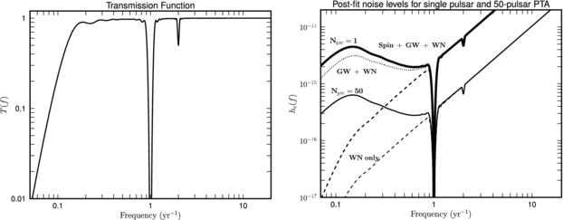
Figure 1. Left: transmission function T(f) for fluctuation power due to standard least-squares fitting to timing data for spindown parameters (fs and  ) and astrometric parameters, including parallax. A unity value means that the power is unaffected by the fit. The 'valley' at the left is from the spindown-polynomial fitting terms while the dips at 1 and 2 yr−1 are due to position and parallax fitting. Right: post-fit level of noise variations expressed as the dimensionless strain hc(f) per unit log frequency. The plotted curves represent only the noise in timing residuals and do not include any true signal (e.g. from the Earth-term GW perturbation). Where noted, they do include the pulsar GW terms, which act as a source of noise. Solid lines show the combined spectrum of noise processes that contribute to timing residuals of a single MSP and a PTA with 50 MSPs. The dotted curve for Npsr = 1 includes GWs (pulsar term) combined with white noise only. The dashed lines show the equivalent curves if only white noise is present in the timing residuals. The curves are only representative and do not indicate the sensitivity of any particular PTA.
Download figure:
Standard image High-resolution image4.1. Other effects
Several effects cause TOA precisions to exceed the theoretical minimum from MF. Amplitude and phase jitter of single pulses was mentioned earlier, along with fast and slow changes in the multipath PBF. Additional effects include clock errors at individual radio observatories (described elsewhere in this issue) and polarization calibration errors, both of which will be epoch dependent in non-obvious ways. Pulsars are often highly polarized so precision polarization calibration is needed to avoid pulse-shape changes that perturb TOAs [19].
5. Correctability of TOAs and spin variations
Current work includes efforts to make higher-order corrections of TOAs and torque variations by investigating pulse shape variations. 'Descattering' of pulse shapes aims to coherently deconvolve the interstellar PBF from the measured signal [4], which will remove the mean delay ∼τd and any epoch-to-epoch variations in τd. Some canonical pulsars show variations in torque that correlate with pulse shape changes on time scales of weeks to months. To varying degrees of precision, the torque changes can be removed from timing data [11]. Similar phenomena have not yet been seen in MSPs, either because the underlying physics is different or because MSPs have not been investigated on pulse-to-pulse time scales to the extent that CPs have. Lastly, amplitude and phase jitter of single pulses also is amenable to correction by exploiting any correlation between TOA variations and jitter-induced stochastic shape changes [6, unpublished notes]. To achieve significant improvement in TOA precision, the correlation coefficient ρ between a pulse shape parameter and TOA perturbations needs to be high. The reduction factor in rms TOA is  , so a 50% reduction requires
  [6, unpublished notes]. Use of multiple shape parameters alters the expression but the basic point remains the same. Recent work [13] indicates ∼20% improvement and has been extended to ∼40% [20]. The degree of improvement depends on the statistics of jitter and seems to rely on an asymmetric phase-jitter distribution (unpublished work).
6. Prognosis for GW detection with PTAs
Current PTA limits on stochastic GW backgrounds approach predictions based on mergers of SMBH binaries yet are based largely on the previous generation of digital spectrometers. New, larger-bandwidth spectrometers combined with new algorithms will yield significantly better sensitivities and will provide constraining limits or detections of the stochastic background, of continuous wave sources (individual SMBH binaries or cosmic strings), or of bursts. The inherent nonstationarity of some of the GW signatures in timing residuals implies growth in signal levels as ∼T5/3 (stochastic background) and ∼T for bursts with memory [2]. However, red spin noise also increases with data span (rms ∝T2, cf equation (4)), so long-term projections depend on the uncertainty in the population average scaling law for spin noise and also on object-to-object differences. Nonetheless, analyses that combine measurements of multiple MSPs to detect the Earth term of the GW perturbation benefit from the  reduction of noise levels. Based on several studies of detectability (Siemens, this volume) and [3], some general statements can be made about prospects for detection of a stochastic background. In most analyses, the detection significance is defined as
  where C is a cross correlation parameter that exploits the correlated Earth term and σC is its error. When σC is dominated by non-GW noise, Sd is said to be noise limited. In the opposite case, it is GW dominated.
- (i)Increasing the number of MSPs (NMSP) helps in any regime, but has greater impact in the noise limited case (rn or wn) where the detection significance Sd is linear in NMSP. In the extreme case where the residuals are GW-dominated, Sd increases only as the
 [3]. Detection of GWs almost certainly will occur in the regime where Sd has a shallower than linear dependence on NMSP.
 - (ii)In the wn-limited regime larger Sd can be obtained through a combination of more pulsars, as above, greater timing throughput (higher cadence and longer integration times), smoothing, and a decrease in timing error per TOA.
- (iii)Because red noise is spectrally similar to the GW contribution and does not average out significantly in temporal correlation functions because of its long correlation time, the primary means for increasing Sd is to sum detection statistics over many pulsars.
- (iv)In the GW-dominated regime increasing the number of pulsars NMSP is the only option.

Acknowledgments
I thank D Madison for providing some of the code used to make figure 1 and to my NANOGrav and IPTA colleagues for many fruitful discussions. Comments from the referees improved the presentation. This work was supported by an NSF PIRE grant to Cornell University.
Footnotes
- 1
Strictly speaking, this should be pulse phase because the apparent pulse period differs from the spin period by the Doppler shift from radial motion of the pulsar.