

Abstract
A feasible design for a magnetic diagnostics subsystem for eLISA will be based on that of its precursor mission, LISA Pathfinder. Previous experience indicates that magnetic field estimation at the positions of the test masses has certain complications. This is due to two reasons. The first is that magnetometers usually back-act due to their measurement principles (i.e., they also create their own magnetic fields), while the second is that the sensors selected for LISA Pathfinder have a large size, which conflicts with space resolution and with the possibility of having a sufficient number of them to properly map the magnetic field around the test masses. However, high-sensitivity and small-sized sensors that significantly mitigate the two aforementioned limitations exist, and have been proposed to overcome these problems. Thus, these sensors will be likely selected for the magnetic diagnostics subsystem of eLISA. Here we perform a quantitative analysis of the new magnetic subsystem, as it is currently conceived, and assess the feasibility of selecting these sensors in the final configuration of the magnetic diagnostic subsystem.
Export citation and abstract BibTeX RIS
1. Introduction
The eLISA mission concept is a proposed spaceborne gravitational wave observatory for the L3 theme 'The gravitational Universe' (ESA) [1]. Its main purpose is the study of the gravitational Universe in the frequency interval between  and
and  . The eLISA concept is based on three drag-free spacecraft in a one-million kilometer side equilateral triangle. Each arm forms a laser interferometer between free-falling bodies (46 mm-side gold-platinum cubes) to measure the weak deformation of spacetime along one arm of the interferometer relative to the other [2]. Due to the extremely low amplitude of gravitational waves [3], the test masses (TMs) are required to be shielded from non-gravitational forces, which would disturb their pure geodesic motion. Consequently, environmental conditions around the TMs need to be under stringent control, otherwise the different noise disturbances would prevent the detection of gravitational waves.
The eLISA noise requirement in terms of free-fall accuracy is  per TM down to 0.1 mHz [2]. At frequencies below 1 mHz, the noise is dominated by the residual acceleration noise caused by environmental effects, e.g., thermal, magnetic and random charging fluctuations [4]. Among them, one of the main contributors to the total acceleration noise budget is the surrounding magnetic field in the spacecraft, which is mostly created by electronic units and other components such as the micro-thrusters of the satellite. The magnetic field and magnetic field gradient can cause a non-gravitational force on the TM due to its non-zero magnetization M and susceptibility χ. This spurious force on the TM volume V induced by a magnetic disturbance is given by:

While the magnetic properties of the TMs ( and χ ) are known owing to several on-ground and in-flight experiments [5, 6], the magnetic field environment (
 and
and  ) at the TM locations needs to be carefully evaluated during the mission. To that end, eLISA will have a set of magnetic sensors placed in key locations, with the purpose of discerning the magnetic noise contributions from the overall acceleration noise budget. The ongoing research concerning the possible design of a magnetic diagnostics subsystem for eLISA is based on the experience with its precursor mission, LISA Pathfinder, in which high-performance fluxgate magnetometers were chosen because of their sensitivity and availability for space applications [7, 8]. However, these sensors are bulky (
 ) and have a large ferromagnetic sensor head (
 long). These reasons led to the placing of only four tri-axial sensors at somewhat large distances from the TMs (
 ) to avoid back-action disturbances. Besides, the size of the sensor head also conflicts with the space resolution, which might be another source of error in the determination of the magnetic field. A view of the magnetometer location in the LISA Pathfinder payload is shown in figure 1.

Figure 1. The payload of LISA Pathfinder, with the four tri-axial fluxgate magnetometers. Each of the electrode housings (cubic structures) inside the vacuum enclosure (the two cylindrical towers) encloses one TM at its center (solid gold cube).
Download figure:
Standard image High-resolution imageWe stress that unlike critical drag-free technology that needs from the in-flight experiments to be fully proved, the feasibility of the magnetic measurement subsystem can be verified in-depth from the analysis of the ground test campaigns. On the basis of the previous analysis for LISA Pathfinder, the selected arrangement of magnetic sensors resulted in an unsatisfactory estimation of the magnetic field in the TM region using classical interpolation methods. Accordingly, alternative approaches needed to be adopted. In particular, an interpolation scheme based on neural networks needed to be developed [9]. For the case of eLISA, a more robust method to reconstruct the magnetic field at the position of the TMs is foreseen. This requires a sufficient number of smaller magnetometers, which additionally must be placed closer to the TMs. Besides, it is required that back-action effects should be negligible. All this has motivated the study of alternatives to fluxgate magnetometers. Specifically, magnetoresistances [13] or chip-scale atomic vapor cell devices [14] have been proposed. These high-sensitivity and small sensors will significantly mitigate the limitations mentioned above. Thus, they will likely be chosen to be integrated in the magnetic diagnostics subsystem in eLISA, improving the quality of magnetic field interpolation.
All in all, the LISA Pathfinder magnetic diagnostics are fully integrated in the spacecraft due to launch in 2015, and the mission operations together with the data analysis are expected to be completed by 2016. Regarding the magnetic interpolation process to be used in LISA Pathfinder, the aforementioned neural networks algorithms is at present the most promising one, although it is still an ongoing activity. On the other hand, eLISA is currently under the mission concept study and the critical technologies need to be be available for the mission concept selection in 2020. Details can be found in [15] regarding the general status of eLISA and its precursor LISA Pathfinder.
In this paper we assess the feasibility of using anisotropic magnetoresistance sensors (AMRs) for estimating the magnetic field and its gradient at the location of the TMs. The article is organized as follows. In section 2 the theoretical methods for the magnetic field interpolation are explained, while in section 3 the sensor array and the distribution of the magnetic sources are addressed. The results of our analysis are presented in section 4. Finally, we draw our conclusions in section 5.
2. Interpolation methods
The magnetic field at the TM location must be inferred according to the information given by the magnetometer readings. We are interested in a robust method that works without previous knowledge of the spacecraft magnetic field environment. The reasons for this choice are that the expected local spacecraft field might be affected by possible changes of the magnetic characteristics of the spacecraft during launch or during the lifetime of the mission, by deviations from the on-ground performance, and by varying operational modes in the spacecraft. Hence, methods making use of 'a priori' knowledge, such as neural networks or Bayesian frameworks that yield remarkable results in similar estimation problems [9–11] will not be considered here. Instead, in this work we adopt as our interpolation tool the multipole expansion technique based only on the magnetometer readouts. The results obtained using this method are then compared with other theoretical approaches, such as the Taylor series and the distance weighting interpolating methods. In the following sections we briefly describe the interpolation methods employed for this study.
2.1. Multipole expansion
Since the magnetic sources in the spacecraft are located far from the origin of the coordinate system (chosen at the center of the TM) and assuming the material inside the vacuum enclosure is basically non-magnetic, the magnetic field in this region can be considered to be essentially a vacuum field ( ). Hence, the estimated magnetic field
  obtained employing an array of N sensors can be written as the general solution to Laplace's equation centered at the TM, which can be expressed in terms of an expansion in spherical harmonics:

where  and
and  are the spherical coordinates of the field at
  . Mlm and Ylm are the multipole coefficients and the standard spherical harmonics of degree l and order m, respectively [12].
The accuracy of the estimation of the magnetic field is given by the order of the expansion, which depends on the number of multipole coefficients that can be computed. Specifically, the accuracy of the interpolation is given by the number of known magnetic field measurements at the boundary of the volume where the field equations are considered. In our case these measurements are provided by the number of magnetometers placed in the spacecraft. Table 1 shows the minimum number of magnetometers required to model the magnetic field with a second, third and fourth order multipole expansion.
Table 1.
Order of the multipole expansion, number of multipole coefficients and number of needed magnetometers. The number of triaxial magnetometers (last column) necessary to achieve the desired order satisfies the condition  .
.
| Expansion | Equivalent | # of Mlm | # of triaxial |
|---|---|---|---|
| order | multipole | coefficients | magnetometers |
| L | [L (L + 2)] | [N] | |
| 2 | Quadrupole | 8 | 3 |
| 3 | Octupole | 15 | 5 |
| 4 | Hexadecapole | 24 | 8 |
The coefficients Mlm are found by minimizing the equation  , where the square error is defined as

 is the readout of the triaxial magnetometer, and N is the total number of magnetometers. This is done employing a least-squares method. Once the system of equations is solved, the computed coefficients Mlm can be inserted into equation (2), replacing the magnetometer's position,
  , by the TM position,
  , to finally obtain the value of the interpolated field at the TM location.
2.2. Taylor series
The magnetic field at the TM position inferred from the readings of the magnetometers can also be approximated by a Taylor expansion. As in the case in which the multipole expansion is employed, the order of the Taylor series is determined by the number of magnetometer data channels. In this case the magnetic field at the position of the TMs can be approximated by the following expression:

where the origin of coordinates is defined at the center of the respective TM ( ), and
  are the magnetometer locations.
  and
and  are calculated considering that the magnetic field around the TM has both zero divergence and curl, i.e. the magnetic field gradient tensor
  is a symmetric and traceless matrix. Thus, only a total of five independent components need to be computed.
2.3. Distance weighting
This method consists of computing the field as a weighted sum of the different magnetometer readings. The calculation is performed as follows:

where  are the readouts of the magnetometers. The weighting factors as are given by:

where n specifies the order of the interpolation and ri are the distances between the point at which the field must be estimated and the specified magnetometer.
3. Magnetic sources and sensor layout
We first note that the interplanetary DC field is expected to be more than one order of magnitude weaker than the sources of magnetic field present inside the spacecraft [16]. By design, there are not any sources of magnetic field inside the vacuum enclosure cylinder. Since the distribution of the different subsystems in eLISA is not fully defined yet, the distribution of the magnetic sources in the spacecraft is not known. However, in order to provide a realistic scenario to assess the performance of our proposed interpolation methods, we make the following assumptions. We first assume that the magnitude and location of the magnetic sources are the ones measured for LISA Pathfinder. Moreover, we also assume that the sources of magnetic field can be modeled as point magnetic dipoles. With these assumptions a batch of 103 different magnetic realizations is generated using the fixed locations and magnitudes of the magnetic field of the sources, but with orientations randomly drawn according to normal distributions for each of the components.
The adequate location and number of magnetometers stems from a trade-off between the accuracy of the reconstruction of the magnetic field map and the magnetic disturbances generated by the magnetometer itself on the TM region. In order to quantify the effect of the sensors, the magnetic moment of an AMR has been measured with a superconducting quantum interference device (SQUID) for different configurations. Our analysis based on the SQUID measurements shows that symmetrical placements with four and eight sensors are the preferred options in order to minimize the magnetic back-action effects. Moreover, when eight sensors are allocated in a symmetrical configuration on the walls of the vacuum enclosure, their contribution to the magnetic budget is negligible [17, 18]. Figure 2 displays the distribution of the sources of the magnetic field in the LISA Pathfinder spacecraft and the eight-sensor layout that is being considered in the current analysis for eLISA. Additionally, we carried out noise measurements of the magnetometer with the sensor allocated inside a magnetic shield, and obtained a noise floor of  [13]. Accordingly, to mimic the electronic noise of the system, this noise is added to the simulated readouts of the magnetometers.
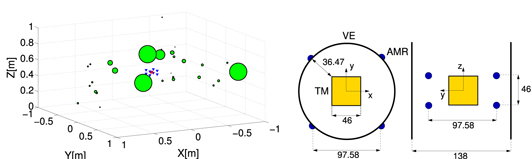
Figure 2. Left: a view of the 29 measured dipole magnetic sources (green dots: the size is proportional to their magnetic moment), the test mass (red square) and the eight AMR magnetometers (blue triangles). Right: sensor array configuration on the vacuum enclosure (units in mm).
Download figure:
Standard image High-resolution imageFinally, in order to assess the performance of each of the interpolating methods, the interpolated magnetic field is compared with the exact one, assuming that the different magnetic sources behave as point dipoles. Then, the total magnetic field generated by the sources can be calculated as:

where  are the magnetic dipolar moments measured for the different subsystems,
  are the source positions and n is the number of sources. The corresponding expression for the magnetic field gradient is:

where  is Kronecker's delta.
4. Results
4.1. Magnetic field reconstruction
As previously explained, to validate the performance of the reconstruction algorithm, a batch of dipoles with randomly generated orientations were simulated and the exact magnetic field for each one of these realizations was compared with the interpolated results. The left panel of figure 3 shows the x-component of the magnetic field map produced by one of these random configurations. The results are then compared in the right panel with those obtained using one of our interpolating methods, in this case the magnetic field reconstructed using multipole expansion. As seen in section 2, a multipole expansion based only on eight triaxial magnetometers readings is able to resolve the magnetic field up to the hexadecapole structure, by computing 24 terms in equation (2). Overall, the field qualitatively resembles the exact one, although there are apparent differences far from the positions of the TMs. However, note that the success of the reconstruction method is determined by the accuracy achieved at the region of interest, i.e. at the TM locations. We perform a more quantitative analysis for the three components of the field below.
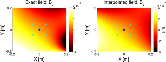
Figure 3. Contour plot of the exact (left) and reconstructed (right) magnetic field Bx for a given source dipole configuration using multipole expansion with eight magnetometers. The positions of the eight magnetometers (cyan triangles) and of the test mass (blue circle) are also represented.
Download figure:
Standard image High-resolution imageThe differences (in percentage) between the interpolated field and the source dipole model field are shown in figure 4. Contour plots for the three components and the modulus show the accuracy achieved by the multipole algorithm. As can be seen in this figure, the smallest differences occur in the region enclosed by the magnetometers. Moreover, the accuracy of the interpolating algorithm is good in the central area of the electrode housing, where the TM is located.

Figure 4. Relative errors in the estimation of the magnetic field components and the modulus. To calculate the relative error for each field component, the absolute error is divided by the modulus of the exact value in order to avoid infinities when one of the vector components is close to zero  .
.
Download figure:
Standard image High-resolution imageTo further confirm the validity and general applicability of the multipole expansion, we compared the differences between the interpolated and exact magnetic field at the position of the TM for three different sensor layouts. Specifically, we first adopted the LISA Pathfinder configuration. In this layout fluxgate magnetometers are used, as depicted in figure 1. In a second step we did the same, adopting four AMRs placed around the vacuum enclosure at the height of the electrode housing center. Finally, we carried out the same calculation, this time adopting eight AMRs, as graphically displayed in figure 2. Average and maximum field errors relative to the modulus ( and
and  ) and to the field components (
 ) over the 103 random runs are shown in table 2. In the LISA Pathfinder configuration the accuracy of the reconstructed field at the TM is poor and presents large variations when the multipole expansion is used. In particular, the estimation errors can be as high as
  . This is the natural consequence of having placed the sensors too far from the center of the TM. Instead, when AMRs are used, the sensors can be placed much closer to the center of the TM, due to its smaller size and intrinsic magnetic moment. The results when the same number of magnetometers is employed show significant improvements, with maximum errors up to 15%. Finally, the estimation errors are reduced by a factor of ∼6 (
 ) when eight sensors are used. In this case the hexadecapole expansion can be employed, and this obviously results in an improved performance of the interpolating algorithm. Last, in figure 5 the distribution of the estimation errors for the randomly simulated cases is shown. This figure clearly shows that the standard deviations are
  and
and  for the 4-AMR and 8-AMR layout, respectively. This proves that the averaged estimation errors (
 ) are robust and that the performance of the multipole interpolating algorithm is good, providing reliable estimated values of the magnetic field at the location of the TM.
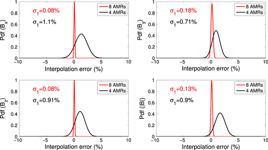
Figure 5. Distributions of the relative errors at the TM position for  random cases for four (black) and eight (red) AMR sensors.
Download figure:
Standard image High-resolution imageTable 2.
Relative errors of the magnetic field estimation at the positions of the TM.  and
and  are the mean error for a batch of 103 randomly orientated magnetic sources relative to the modulus
  and to the field component
  , respectively. The denominator in
  is closer to zero than that of the modulus
  , and this translates in larger errors for the x-component than for the modulus.
| Error | LPF (4 fluxgates) | eLISA (4 AMRs) | eLISA (8 AMRs) | |||||||||
|---|---|---|---|---|---|---|---|---|---|---|---|---|
( ) ) |
Bx | By | Bz |

|
Bx | By | Bz |

|
Bx | By | Bz |

|

|
38.2 | 28.1 | 20.9 | 32.5 | 1.4 | 1 | 1.1 | 1.8 | 0.1 | 0.2 | 0.1 | 0.1 |

|
737.7 | 340.3 | 327.6 | 803.2 | 15.0 | 7.7 | 14.0 | 13.3 | 0.9 | 2.4 | 1.4 | 2.0 |

|
697.9 | 202.1 | 184.5 | 32.5 | 13.7 | 3.8 | 7.8 | 1.8 | 0.6 | 0.8 | 5.3 | 0.1 |
The results described so far were obtained using the multipole expansion algorithm. However, other interpolation schemes were detailed in section 2, and their performance compared with that of the multipole expansion in table 3. The order of the interpolation in the distance weighting method is set to n = 1. Nevertheless, this choice is not relevant due to the physical symmetry of the sensor placement, i.e., the distances rs, and consequently the weighting factors as, are equivalent for the eight magnetometers. For the Taylor expansion, the second and the terms involving higher-order derivatives are negligible due to the symmetry of the magnetic distribution. Thus, the Taylor approach mainly estimates the magnetic field as a linear approximation. For this reason, we expect the results of the interpolation to be almost identical to those obtained using the distance weighting method. Table 3 shows the accuracies of the estimation of the magnetic field at the position of the TM for the three methods employed in this work. As can be seen, the multipole expansion outperforms by far the rest of the methods described previously.
Table 3. Maximum errors of the estimated magnetic field at the position of the TM using different interpolation methods, see text for details.
![${\varepsilon }_{| {\bf{B}}| ,\mathrm{max}}\;[\%]$](https://content.cld.iop.org/journals/0264-9381/32/16/165003/revision1/cqg516542ieqn53.gif)
|
||||
| Error | Bx | By | Bz |

|
| Distance weighting | 8.0 | 4.0 | 7.7 | 7.9 |
| Taylor expansion | 8.0 | 4.0 | 7.7 | 7.9 |
| Multipole expansion | 0.9 | 2.4 | 1.4 | 2.0 |
4.2. Reconstruction of the magnetic field gradient
Magnetic field gradients also need to be estimated from the readouts of the eight AMRs. We do this using the multipole expansion algorithm because, as demonstrated earlier, this interpolating method outperforms the other two methods studied here. For the sake of clarity, only the errors of the gradient interpolation for two components ( and
and  , respectively) along the spacecraft are shown in figure 6. In this case, minimum errors are also obtained in the center of the TM, though unlike that obtained for the case of the magnetic field, the error increases somewhat faster in the region outside of the boundary of the area surrounding the magnetometers. Additionally, relative errors around the TM area are slightly larger than those found for the reconstruction of the magnetic field, although they remain lower than 3%. Figure 7 shows the distribution of the estimation errors and standard deviations for five independent components of the gradient matrix
  at the position of the TM. Inspection of this figure reveals that the multipole expansion scheme is robust. In particular, when this interpolant is used, we obtain not only accurate values of the reconstructed magnetic field, but also of its gradient, with typical accuracies of the order of 2%, and deviations below
  respectively.
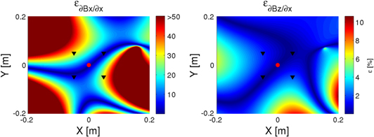
Figure 6. Relative errors in the estimation of the magnetic field gradient. Here, for the sake of clarity, we only show two components,  and
and  . The relative error is computed as
  . Note the different scale for the error bars.
Download figure:
Standard image High-resolution image
Figure 7. Probability density function of the relative errors at the TM position for 103 random cases. Five independent terms in the field gradient matrix ( ,
,  ,
,  ,
,  and
and  ) are considered. Standard deviations and averaged errors relative to the modulus (
 and
and  ) are shown.
Download figure:
Standard image High-resolution image4.3. Other sources of error
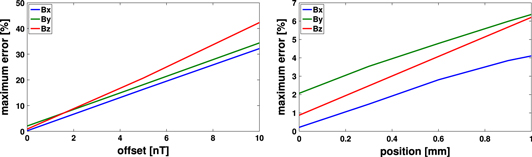
Absolute errors and drifts of the magnetometers readings are relevant to the interpolation quality, since the algorithm is entirely based on the magnetometer outputs. Due to the stringent stability requirements for eLISA, drifts of the measurements are not critical. Thus, the analysis is focused on the absolute errors. To validate the robustness of the system, the performance of the multipole expansion scheme is studied for two common sources of error. Namely, possible offsets in the magnetometer readings and spatial uncertainty—that is, deviations from the nominal position of the sensor core. We analyze their eventual effects separately. Offsets in the magnetometer or in the signal conditioning circuit can be measured on-ground and considered in the analysis. However, unknown magnetometer offsets due to launch stresses can lead to inaccurate field determination [19]. The precision of the position of the sensors may eventually be another source of error that cannot be ignored 'a priori'. The spatial uncertainty depends on the size of the sensor head, since smaller heads result in a smaller uncertainty of the precise location of the measurement.
The offsets of the magnetometers can be relevant depending on the measurement technique. In particular, for AMR sensors, flipping signals applied to the sensor help to overcome the offset by reversing the sensor magnetization and modulating the output signal [20]. The changes in the direction of the sensor magnetization lead to inversion of the output characteristics but not the offset, which can be canceled by subtracting the measurements between each flipping pulse. Regarding the spatial uncertainty, the layout of the thin film forming the AMR Wheatstone bridge [21] is deposited by a sputtering process, and has a rough area of  . Therefore, a spatial uncertainty smaller than
  is expected.
The impact of these effects on the accuracy of the multipole expansion algorithm is simulated as follows. First, a  matrix of offsets is randomly generated according to a uniform distribution with an interval of
 ![$[-{B}_{\mathrm{Offset}},{B}_{\mathrm{Offset}}]$](https://content.cld.iop.org/journals/0264-9381/32/16/165003/revision1/cqg516542ieqn72.gif) . Second, the offset array is added to the
. Second, the offset array is added to the  magnetic channels readings, and finally the magnetic field and errors are estimated. These steps are sequentially repeated for series of 103 random offsets with intervals of the same length. A similar procedure is done to assess the robustness of the interpolation to the uncertainty in the location of the sensor heads. The maximum estimation errors as a function of the offset and of the spatial uncertainty are shown in figure 8. As can be observed, the offset of the sensor is more determinant than its spatial resolution. Specifically, for an unpredictable non-measured offset of
  , the maximum estimation error is
  . These results reflect the relevance of the magnetic sensing technology. Specifically, we stress that appropriate techniques to cancel out the undetermined offset and the use of tiny sensors with accurate spatial resolution are totally necessary.
Figure 8. Maximum estimation error of the magnetic field as a function of the offset (left) and spatial uncertainty (right) of the magnetometer.
Download figure:
Standard image High-resolution image
5. Conclusion
An AMR-based magnetic diagnostics subsystem for eLISA has been presented as an alternative to the one using fluxgates in LISA Pathfinder. This new design leads to a reliable estimation of the magnetic field and its gradient at the positions of the test masses. Actually, the multipole expansion scheme used in combination with the proposed eight-sensor configuration will represent a reduction of the magnetic field estimation error of more than two orders of magnitude when compared to the solution implemented in LISA Pathfinder. Besides, we have shown that the estimation errors computed for different simulated magnetic scenarios employing the multipole expansion interpolation provide a robust algorithm that does not need any 'a priori' knowledge of the magnetic structure in the spacecraft. Also, in addition to these significant advantages, the proposed system has the ability to deliver correct results under unpredictable offsets of the magnetometer readings, and to overcome reasonable imprecisions in the spatial location of the magnetometers. All in all, these improvements in the accuracy of the magnetic field reconstruction are achieved due to the smaller size and smaller magnetic back-action of the AMR sensors, which enable more sensors to be placed and for them to be located closer to the TMs. This is a promising result that proves that the use of AMRs combined with the multipole expansion will provide a reliable estimate of the magnetic characteristics at the positions of the test masses of eLISA.
Acknowledgments
We are grateful to Airbus Defence and Space for providing the measured magnetic moment values for the LISA Pathfinder units. Support for this work came from grants AYA2010-15709 and AYA2011-23102 of the Spanish Ministry of Science and Innovation (MICINN), ESP2013-47637-P of the Spanish Ministry of Economy and Competitiveness (MINECO), and 2009-SGR-935 (AGAUR). This work was partially supported by the European Union FEDER funds.