
Abstract
The first observing run of Advanced LIGO spanned 4 months, from 12 September 2015 to 19 January 2016, during which gravitational waves were directly detected from two binary black hole systems, namely GW150914 and GW151226. Confident detection of gravitational waves requires an understanding of instrumental transients and artifacts that can reduce the sensitivity of a search. Studies of the quality of the detector data yield insights into the cause of instrumental artifacts and data quality vetoes specific to a search are produced to mitigate the effects of problematic data. In this paper, the systematic removal of noisy data from analysis time is shown to improve the sensitivity of searches for compact binary coalescences. The output of the PyCBC pipeline, which is a python-based code package used to search for gravitational wave signals from compact binary coalescences, is used as a metric for improvement. GW150914 was a loud enough signal that removing noisy data did not improve its significance. However, the removal of data with excess noise decreased the false alarm rate of GW151226 by more than two orders of magnitude, from 1 in 770 yr to less than 1 in 186 000 yr.

Original content from this work may be used under the terms of the Creative Commons Attribution 3.0 licence. Any further distribution of this work must maintain attribution to the author(s) and the title of the work, journal citation and DOI.
1. Introduction
The Advanced Laser Interferometer Gravitational-Wave Observatory (aLIGO) is comprised of two dual-recycled Michelson interferometers [1] located in Livingston, LA (L1) and Hanford, WA (H1). A gravitational wave passing through a LIGO interferometer will induce a strain on spacetime, stretching and squeezing the 4 km arms and generating an interferometric signal at the antisymmetric port of the beamsplitter.
Advanced LIGO's first observing run (O1) lasted from 12 September 2015 to 19 January 2016. A primary goal of this observing run was the detection of gravitational waves from compact binary coalescences (CBC) [2]. This goal was achieved with the detections of GW150914 and GW151226, both signals from binary black hole systems, which marked the first direct detections of gravitational waves [3, 4]. These detections were part of a broader search for CBC signals carried out by multiple search pipelines during O1 [5–10] and searches for unmodeled transients [11–14].
Searching for gravitational waves requires an understanding of instrumental features and artifacts that can adversely affect the output of a gravitational wave search pipeline. Throughout the observing run, noisy data were identified in the form of data quality (DQ) vetoes to ensure that the analysis pipelines did not analyze data known to be contaminated with excess noise [15]. These vetoes are discussed further in section 4. This study measures the effects of removing data with excess noise on the output of PyCBC [5, 9, 10], a python-based pipeline used to search for CBC signals. Section 3 contains a brief description of the PyCBC search pipeline and its internal DQ features.
Section 2 outlines the data selection and noise characterization processes. The DQ vetoes that are generated in the noise characterization process are described in section 4. The methodology of this study is discussed in section 5. This paper focuses on two specific subsets of the O1 data set. The first data set, from 12 September–20 October 2015, was used for background estimation for GW150914. This data set is discussed in section 6. The second data set, from 3 December 2015–19 January 2016, was used for background estimation for GW151226. This data set is discussed in section 7. Section 8 describes the limiting noise sources for CBC searches.
2. Data selection
The strain data measured at the output of the detectors are typically non-stationary and non-Gaussian and contain noise artifacts of varying durations. The longer duration non-stationary data can affect the overall sensitivity of the search, but they do not result in loud background events as they occur on a timescale of hours. The transient noise artifacts, however, occur on a timescale of seconds and can reduce the sensitivity of CBC searches by producing loud background events.
Data quality studies must be performed to search for causes of transients in the data that generate loud events in a gravitational wave search. If the source of noise is identified, a veto is generated to flag times when transient noise makes the data unsuitable for analysis. Section 4 describes DQ vetoes that are used to indicate when the detector data are known to have excess noise [15–18]. The exception to this process is gating [5], which is a feature internal to the CBC searches. This gating, which is applied independently of DQ vetoes, uses a window function to remove times containing large transients from the input data stream.
3. The PyCBC search pipeline
The PyCBC pipeline is designed to search for gravitational wave transients from CBCs [5]. It employs a matched filter algorithm, which correlates expected CBC waveforms with detector data and outputs a ranking statistic, the signal-to-noise ratio (SNR). If the ranking statistic exceeds a specified threshold, an event, or 'trigger', is generated. The SNR of each trigger is weighted based on a signal consistency test [19], resulting in a refined ranking statistic called re-weighted SNR. Section 3.1 discusses this signal consistency test further.
To perform this search, the matched filter algorithm needs to know what to search for. A collection of model CBC waveforms is generated before the analysis [20, 21]. Each of these waveforms is called a template and the full collection of waveforms is referred to as the template bank. This template bank is constructed to span the astrophysical parameter space included in the search [22]. Each waveform is defined by the mass and spin of each compact object in the binary system. It is often convenient to combine the effects of each object's spin into one parameter called effective spin , which is the mass-weighted spin of the system [7]. The mass of the binary system is often represented by the chirp mass [23], which is used to parameterize gravitational wave signals in general relativity.


The search algorithm is run separately at each detector and a set of single detector triggers is generated. The two sets of single detector triggers are then compared to search for any events that were recorded within a 15 ms coincidence window, which reflects the travel time of a gravitational wave between the detectors and allows for uncertainty in the arrival time of a signal [5]. Any triggers that are found in coincidence with the same source parameters in both detectors represent potential gravitational wave signals and are referred to as foreground events. Some of these foreground events will be chance coincidences between noise in each detector, which is expected given the number of events in each data set.
To determine the statistical significance of foreground events, a background distribution is generated using a time shift technique [5]. The statistical significance of any candidate gravitational wave is then quantified by calculating the rate of background events from detector noise that are at least as loud as the candidate event. This statistic is called the false alarm rate (FAR). Any loud triggers that appear as the result of instrumental transients will extend the background distribution and the influence the measured false alarm rate. The purpose of the DQ effort as a whole is thus two-fold: to ensure that the search is using representative detector data in the background noise estimation and to suppress the rate of loud events that will pollute both the background and the foreground distributions.
3.1. signal consistency test

A further layer of effective DQ that is internal to the PyCBC pipeline is the application of the signal consistency test [19]. The SNR produced by the matched filter is an integral in the frequency domain. The test divides each CBC waveform into frequency bins of equal power, checking that the SNR is distributed as a function of frequency as expected from an actual CBC signal. Each trigger that comes out of the matched filter search is down-weighted based on the results of the test. This is folded into a new ranking statistic for CBC triggers, which is called re-weighted SNR and is denoted by . The ranking statistic for coincident events in the PyCBC search is the network re-weighted SNR, , which is the quadrature sum of the re-weighted SNR from each detector. Since a real signal has a power distribution that matches the template waveform, it will not be down-weighted by the test; the SNR and the re-weighted SNR will be the same.


This test is extremely powerful, as shown in figure 1, which shows the distribution of single detector PyCBC triggers generated from 12 September to 20 October 2015. Figure 1(a) shows the distribution of triggers in SNR. The extensive tail of triggers with high SNR, which extends beyond SNR 100, is down-weighted in the re-weighted SNR distribution, leaving behind a tail that extends to as seen in figure 1(b). This re-weighted SNR tail represents the loudest single detector background triggers in the CBC search. Investigating this set of loudest background triggers guides DQ efforts in defining the current limiting noise sources to the CBC search.


Figure 1. Histograms of single detector triggers from the Livingston (L1) detector. These triggers were generated using data from 12 September to 20 October 2015. These histograms contain triggers from the entire template bank, but exclude any triggers found in coincidence between the two detectors. (a) A histogram of single detector triggers in SNR. The tail of this distribution extends beyond SNR = 100. (b) A histogram of single detector triggers in re-weighted SNR. The chi-squared test down-weights the long tail of SNR triggers in the re-weighted SNR distribution. The triggers found using only the Hanford detector have a similar distribution.
Download figure:
Standard image High-resolution image4. Data quality vetoes
As seen in figure 1, the test is a powerful tool, but there is still a considerable tail in the single detector trigger distribution. This tail is often caused by transient instrumental noise. If these noise sources can be linked to a systematic instrumental cause or a period of highly irregular instrumental performance, they can be flagged and removed from the analysis in the form of a DQ veto.

DQ vetoes indicate times that are unsuitable for analysis or are likely to produce false alarm gravitational wave triggers. These vetoes are constructed by ∼200 000 witness sensors that continuously monitor LIGO detectors and their environment [15]. Before a witness sensor is used to generate a DQ veto, its sensitivity to a genuine gravitational wave signal is assessed to ensure true signals are not unnecessarily removed from analysis. To test this, a gravitational wave signal is simulated by electromagnetically controlling the motion of the detector optics. If a witness sensor is observed to be sensitive to such an injected signal, it will be considered unsafe for generating DQ vetoes.
As an example, a veto was generated during O1 to mark times when an electronics fault caused amplitude fluctuations in the radio frequency (RF) sidebands used to sense and control LIGO's optical cavities. These amplitude fluctuations introduced noise into the feedback loops controlling the motion of the LIGO optics. This excess motion coupled into the output of the detector and created transient, broadband noise artifacts. A witness sensor monitoring the amplitude stabilization control signal for the RF sidebands was found to be correlated to the excess noise in the detector output. A threshold was established to indicate when the amplitude fluctuations were significant enough to couple into the detector output and any times where the fluctuation amplitude exceeded this threshold were marked as unfit for astrophysical analysis. The process of generating this veto is further detailed in appendix A of [15].
Other examples of noise sources that were vetoed in O1 are photodiode saturations, analog-to-digital converter (ADC) and digital-to-analog converter (DAC) overflows, elevated seismic noise, and computer failures. These DQ vetoes were generated using a process similar to that used to veto the RF amplitude fluctuation noise.
DQ vetoes are produced for all analysis time based on systematic instrumental conditions without any regard for the presence of gravitational wave signals. All data are treated equally; the removal of data with excess noise has the ability to remove real gravitational wave signals as well as background events. The same set of DQ vetoes was applied by all CBC searches in O1 and will be released with any public data to ensure that astrophysical results are reproducible. Further details on DQ vetoes applied in the first observing run are available in a paper detailing the transient noise in the detectors at the time of GW150914 [15].
5. Measuring the effects of data quality vetoes
To test the effects of DQ vetoes, the PyCBC search pipeline was run with and without applying vetoes. The only vetoes that were used in all runs are those that indicate that the data were not properly calibrated, that a data dropout occurred, or that there were test signals being injected into the detectors. Gating is internal to the search pipeline and was applied in all of the analyses. Two methods were used to understand the effects of applying vetoes. The first, described in section 5.1, considers the average sensitivity of the search pipeline to gravitational wave signals. The second, described in section 5.2, compares the measured search backgrounds and the false alarm rates of recovered gravitational wave signals.
5.1. Measuring search sensitivity
The metric used to measure the sensitivity of the search pipeline is sensitive volume. Sensitive volume is measured by injecting simulated gravitational wave signals into the data and attempting to recover them using the search [5]. The ability of the pipeline to recover signals at a given false alarm rate is then measured by analyzing the number of missed and recovered injections.
In addition to the sensitive volume, the amount of time used in the analysis must be considered when removing noisy data. If a search is rejecting too much data, it will miss the opportunity to detect signals. To address this, the sensitive volume of the search is multiplied by the amount of analysis time to create a new metric called VT. If time is removed from an analysis, the sensitive volume of the search must increase to make up for the shorter analyzed time.
The sensitivity of a search varies as a function of the significance threshold set for candidate events. The VT ratios are therefore calculated at both the 1 per 100 yr and the 1 per 1000 yr levels. These significance levels are expressed as inverse false alarm rates (IFAR).
5.2. Comparing search backgrounds
In the first observing run, the bank of CBC waveform templates used in the PyCBC search was divided into three bins [22]. The significance of any candidate gravitational wave found in coincidence between the two detectors is calculated relative to the background in its bin. Waveforms with different parameters will respond to instrumental transients in different ways. This binning is performed so that any foreground triggers are compared to a background generated from similar waveforms. As such, the effects of removing data from the PyCBC search are variable depending on which bin is considered. The actual gravitational wave signals discovered in the PyCBC search, GW150914 and GW151226, were part of a full search that was broken into 3 bins but reported as a single table of results. Because of this, their reported false alarm rates include a trials factor of 3. The background distributions shown in sections 6 and 7 were measured on a bin-by-bin basis, so the cumulative trigger rates have not been divided by 3.
The first bin is called the binary neutron star (BNS) bin and contains all waveforms with . The second bin is the edge bin, which is defined based on the peak frequency of each CBC waveform. These waveforms are typically shorter in duration than binary neutron star waveforms and are comprised of both binary black hole (BBH) and neutron star-black hole (NSBH) binary waveforms. Waveforms in the edge bin typically have high masses and negative . In this analysis, the edge bin contained waveforms with Hz. The third bin is the bulk bin, which contains all remaining waveforms needed to span the parameter space of the search. This contains BBH and NSBH waveforms with a variety of mass ratios and spins.


6. Analysis containing GW150914
The analysis containing GW150914 lasted from 12 September–20 October 2015 and contained a total of 18.2 d of coincident detector data. Of this 18.2 d, 7.7% was considered unfit for astrophysical analysis and was removed from the data set.
6.1. Search sensitivity
To measure the effects of DQ vetoes on the sensitivity of the search, the analysis containing GW150914 was performed with and without applying data quality vetoes. The resulting measurements of VT were divided to calculate a VT ratio.
Figure 2 shows the change in VT when vetoes are applied for two values of IFAR and several chirp mass bins. The lowest chirp mass bin contains BNS signals and does not show any improvement in sensitivity when DQ vetoes are applied. This is discussed further in section 6.2. Since the bulk and edge bins contain systems with a large range of masses that can respond in different ways to instrumental artifacts, these higher mass bins have been split for sensitivity estimation. The higher mass bins in figure 2 are binned linearly in ln(). The higher chirp mass bins show an improvement in search sensitivity for both values of IFAR.


Figure 2. The change in search sensitivity when DQ vetoes are applied for the analysis containing GW150914. The error bars show the error from each VT calculation combined in quadrature. The lowest chirp mass bin, which contains BNS signals, does not show any improvement in sensitivity. For marginally significant signals at IFAR = 100, the measured value of VT increases by 3–32% in higher chirp mass bins. For highly significant signals at IFAR = 1000, the measured value of VT increases by 34–62% in higher chirp mass bins.

Download figure:
Standard image High-resolution image6.2. BNS bin
Binary neutron star systems have the longest waveforms used in the search pipelines. Since these signals spend ∼10–100 s in LIGO's sensitive band, the test is effective at discriminating between binary neutron star signals and transient noise, which have a duration of ∼1 s.

Figure 3 shows the background distribution of the BNS bin in the PyCBC search for the analysis containing GW150914. As expected, since waveforms in the BNS bin are not as susceptible to instrumental transients, the background distribution does not change significantly when noisy data are removed from the analysis.

Figure 3. The background distribution in the BNS bin before and after applying DQ vetoes for the analysis containing GW150914. (a) The cumulative rate of background triggers in the BNS bin as a function of re-weighted SNR. (b) A histogram of background triggers in the BNS bin. The red traces indicate the distribution of background triggers without noisy data removed, the cyan traces indicate the distribution of background triggers with all DQ vetoes applied. The BNS bin shows no significant improvement in cumulative rate.
Download figure:
Standard image High-resolution image6.3. Bulk bin
Figure 4 shows the background distribution in the bulk bin for the analysis containing GW150914. If noisy data are not removed from the analysis, there is a shoulder in the distribution that extends to , which limits the sensitivity of the search in the region where 11 .


Figure 4. The background distribution in the bulk bin before and after applying DQ vetoes for the analysis containing GW150914. (a) The cumulative rate of background triggers in the bulk bin as a function of re-weighted SNR. (b) A histogram of background triggers in the bulk bin. The red traces indicate the distribution of background triggers without noisy data removed and the cyan traces indicate the distribution of background triggers with all DQ vetoes applied. When vetoes are not applied, there is a shoulder in the distribution that limits the sensitivity of the search. The dash-dotted line indicates the network re-weighted SNR of LVT151012. The dashed line indicates the network re-weighted SNR of GW150914, which is the loudest event in this bin for both configurations.
Download figure:
Standard image High-resolution image6.3.1. LVT151012.
The second most significant trigger in the analysis containing GW150914 was LVT151012, recorded on 12 October 2015 [22, 24]. This trigger was recovered in the bulk bin with and a false alarm rate of 0.33 yr−1. This is not significant enough to be claimed as a confident detection. The false alarm rate decreases by a factor of 2.1 when DQ vetoes are applied, as shown in table 1.

Table 1. Table of bulk bin false alarm rates for LVT151012.
| Analysis configuration | False alarm rate () |
|---|---|
| All vetoes applied | 0.33 |
| No vetoes applied | 0.69 |

6.4. Edge bin
Figure 5 shows the background distribution in the edge bin for the analysis containing GW150914. There is a visible separation between the two curves that increases for larger values of , indicating that the ability of the search pipeline to make confident detections is diminished in this region.


Figure 5. The background distribution in the edge bin before and after applying DQ vetoes for the analysis containing GW150914. (a) The cumulative rate of background triggers in the edge bin as a function of re-weighted SNR. (b) A histogram of background triggers in the edge bin. The red traces indicate the distribution of background triggers without noisy data removed from the analysis and the cyan traces indicate the distribution of background triggers with all data quality vetoes applied.
Download figure:
Standard image High-resolution image6.4.1. GW150914.
The gravitational wave signal GW150914 was detected on September 14, 2015 with 23.6 [3]. The false alarm rate of GW150914 does not change significantly when noisy data are removed from the analysis, which can be seen in table 2. This is an expected result as GW150914 is louder than the entire background distribution in the bulk bin.

Table 2. Table of bulk bin false alarm rates for GW150914. GW150914 is loud enough that its false alarm rate does not change significantly when noisy data are removed from the analysis. Any change in false alarm rate is due to small changes in the total analysis time after data removal.
| Analysis configuration | False alarm rate () |
|---|---|
| All vetoes applied | < |
| No vetoes applied | < |


7. Analysis containing GW151226
The extended analysis containing GW151226 lasted from 3 December 2015–19 January 2016 and contained a total of 16.7 days of coincident detector data. Of this 16.7 days, 6.5% was considered unfit for astrophysical analysis and was removed from the data set.
7.1. Search sensitivity
Figure 6 shows the change in VT when DQ vetoes are applied to the analysis containing GW151226. For this analysis, the lowest chirp mass bin, which contains BNS signals, shows a slight improvement when vetoes are applied. This improvement is discussed further in section 7.2. Similar to the analysis containing GW150914, the higher chirp mass bins show an improvement in search sensitivity for both values of IFAR.

Figure 6. The change in search sensitivity when DQ vetoes are applied for the analysis containing GW151226. The error bars show the error from each VT calculation combined in quadrature. The lowest chirp mass bin, which contains BNS signals, shows a small improvement in sensitivity when vetoes are applied, though the error bars are consistent with a VT ratio of 1. For marginally significant signals at IFAR = 100, the measured value of VT increases by 27–62% in higher chirp mass bins. For highly significant signals at IFAR = 1000, the measured value of VT increases by 45–90% in higher chirp mass bins.

Download figure:
Standard image High-resolution image7.2. BNS bin
As expected from figure 6, there is a small improvement in the BNS background distribution when DQ vetoes are applied. Figure 7 shows the background distributions in the BNS bin with and without noisy data removed. Although the of the loudest background event does not change considerably, there is a noticeable gap between the two background distributions that is visible at and widens to an order of magnitude difference in FAR at .


Figure 7. The background distribution in the BNS bin before and after applying DQ vetoes for the analysis containing GW151226. (a) The cumulative rate of background triggers in the BNS bin as a function of re-weighted SNR. (b) A histogram of background triggers in the BNS bin. The red traces indicate the distribution of background triggers without noisy data removed and the cyan traces indicate the distribution of background triggers with all vetoes applied.
Download figure:
Standard image High-resolution image7.3. Bulk bin
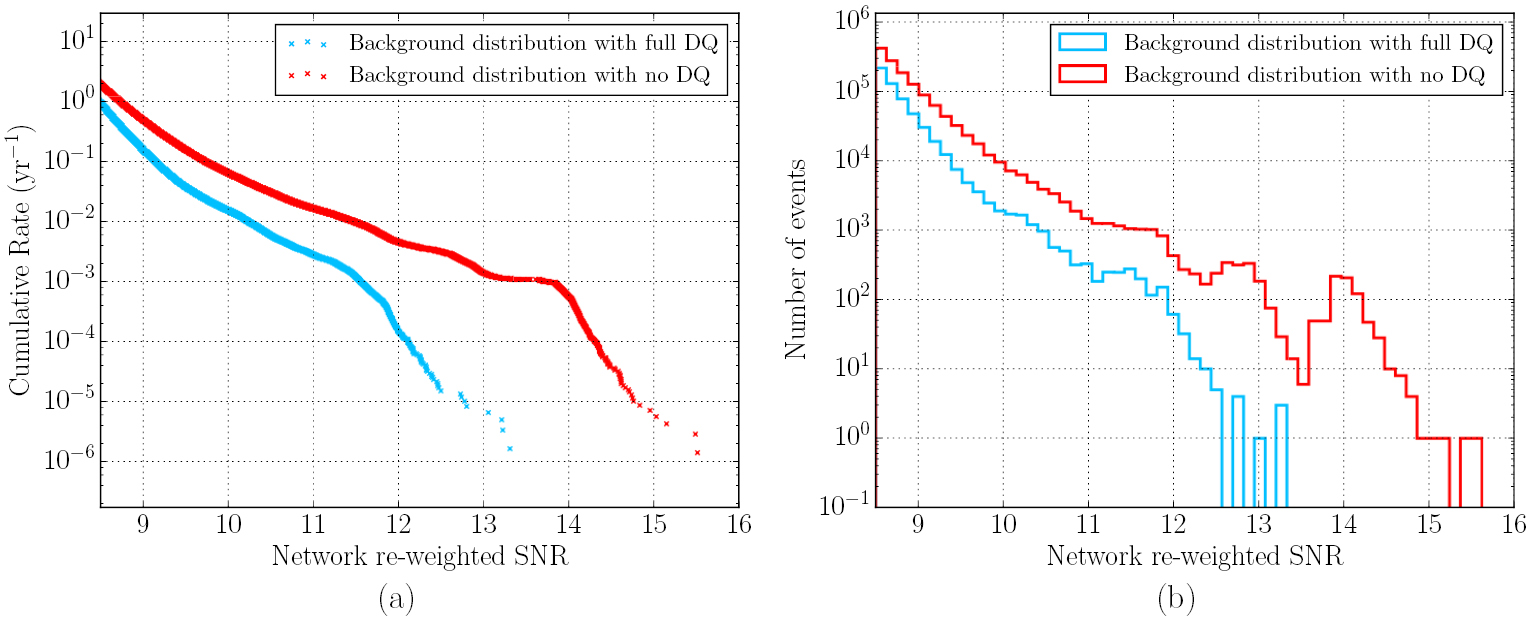
The background distribution in the bulk bin changes significantly when DQ vetoes are applied, which is shown in figure 8. There is a visible difference between the two distributions beginning at . The difference in cumulative rate reaches an order of magnitude at and continues to grow for larger values of . The reduction of the background distribution through the application of DQ vetoes is particularly impactful for GW151226, which is discussed in section 7.3.1.


Figure 8. The background distribution in the bulk bin before and after applying DQ vetoes for the analysis containing GW151226. (a) The cumulative rate of background triggers in the bulk bin as a function of re-weighted SNR. (b) A histogram of background triggers in the bulk bin. The red traces indicate the distribution of background triggers with no data removed from the analysis. The cyan traces indicate the distribution of background triggers with all DQ vetoes applied. The dotted line indicates GW151226, which was recovered with . If DQ vetoes are not applied, GW151226 is no longer louder than the entire background distribution.

Download figure:
Standard image High-resolution image7.3.1. GW151226.
The second binary black hole system discovered in the first observing run, GW151226 [4], is indicated by the vertical dotted line at in figure 8. When noisy data are removed from the analysis, the background distribution in the bulk bin is reduced and GW151226 is the loudest event in the analysis. The false alarm rate of GW151226 decreases by over two orders of magnitude, resulting in a clear detection. The false alarm rates before and after DQ vetoes are applied are listed in table 3.

Table 3. Table of bulk bin false alarm rates of GW151226. The false alarm rate of GW151226 increases from less than 1 in 186 000 yr to 1 in 770 yr if data with excess noise is not removed from the analysis.
| Analysis configuration | False alarm rate () |
|---|---|
| All vetoes applied | < |
| No vetoes applied |


7.4. Edge bin
Figure 9 shows the background distribution in the edge bin before and after DQ vetoes have been applied. The background distribution of the edge bin in the analysis containing GW151226 is significantly reduced for all values of when DQ vetoes are applied.

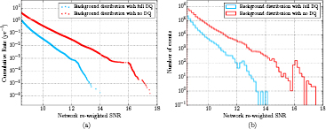
Figure 9. The background distribution in the edge bin before and after applying DQ vetoes for the analysis containing GW151226. (a) The cumulative rate of background triggers in the edge bin as a function of re-weighted SNR. (b) A histogram of background triggers in the bulk bin. The red traces indicate the distribution of background triggers without removing noisy data and the cyan traces indicate the distribution of background triggers with all vetoes applied.
Download figure:
Standard image High-resolution image8. Limiting noise sources
The sensitivity of the search is limited by instrumental features that result in high triggers and tails in the background distributions. This section uses two particular instrumental noise sources from the analysis containing GW150914 as case studies. These are examples of noise sources that are not able to be vetoed using existing algorithms as they are not captured by any existing witness sensors in the detectors.

8.1. Blip transients
Blip transients [15] are band-limited noise transients that occur in both the Hanford and Livingston detectors. They do not occur in coincidence between the two LIGO detectors and are not candidate gravitational wave signals. Due to their short duration in LIGO's sensitive frequency band, the test is not as effective at down-weighting these noise transients and they have been a common source of high re-weighted SNR background triggers. Figure 10 shows a time-frequency representation of a blip transient.


Figure 10. A time-frequency representation [25] of the Livingston strain channel at the time of a blip transient. This visualization of a blip transient demonstrates their typical features: band-limited, short duration, and little visible frequency structure.
Download figure:
Standard image High-resolution imageFigure 11 shows a time-domain representation of a blip transient in the Livingston strain channel. The dotted line on top of the strain data represents a template waveform that reported a high re-weighted SNR at the time of this blip transient. Both curves have been filtered to isolate the parts of the signal that are in LIGO's sensitive frequency band. The template waveform is a high mass system () with an anti-aligned effective spin of −0.97. This waveform is among the shortest duration templates used in the analysis, spending less than 0.1 s in LIGO's sensitive frequency band.


Figure 11. A filtered time-domain representation of the Livingston strain channel at the time of a blip transient. The dotted line is a filtered CBC waveform that reported a high re-weighted SNR value at the time of the blip transient. Both sets of data have been zero-phase bandpass filtered to isolate the frequency range that aLIGO is sensitive to. The short duration and high overlap of these two curves causes the to be ineffective at down-weighting these transients.


Download figure:
Standard image High-resolution imageThe region of the astrophysical parameter space where the test is ineffective at down-weighting blip transients is small. This is demonstrated in figure 12, which shows triggers from the Livingston detector during the analysis containing GW150914. Each point represents the highest single detector re-weighted SNR measured in that region of the parameter space. Figure 12(a) shows this trigger set binned by total mass and effective spin. Templates that overlap with blip transients and produce high re-weighted SNR triggers, such as the template plotted in figure 11, are constrained to the region where and . This region contains only 65 waveform templates out of 249077 total waveforms in the template bank; the majority of the template bank is capable of rejecting blip glitches using the test. Blip glitches that cause loud background events in this region of the template bank populate the tail of the background distribution in the edge bin and limit search sensitivity in that bin.


Figure 12. Single detector triggers from the Livingston detector during the analysis containing GW150914. (a) Triggers binned by total mass and effective spin. The highest re-weighted SNR triggers are constrained to the bottom corner of the plot, bounded by and . (b) Triggers binned by the peak frequency and duration of the template waveform. The loudest triggers in re-weighted SNR are constrained to the area of the parameter space with template durations <0.1 s. The small cluster of loud triggers with a template duration of roughly 4 s corresponds to the 60–200 Hz noise discussed in section 8.2.


Download figure:
Standard image High-resolution imageThe region of the template bank where the test is ineffective can also be visualized in terms of the duration of the template waveform. Figure 12(b) shows the same trigger set binned by the peak frequency and duration of the template waveform. In this view of the parameter space, the templates with the highest re-weighted SNR are contrained to the region where the duration of the template in LIGO's sensitive frequency band is less than 0.1 s. In this region, the duration of the template is on the same time scale as instrumental transients such as blip transients.

Mitigation of blip transients is a high priority but is difficult since they do not couple into instrumental witness sensors and are not high enough in amplitude to be removed by the gating process. Since an instrumental cause has not yet been identified, a modified ranking statistic [26] that is capable of better discriminating blip transients from gravitational wave signals has been developed and implemented for the second observing run.
8.2. 60–200 Hz noise
A second problematic noise source that was present at Livingston during the first observing run was the '60–200 Hz' noise. Figure 13 shows a time-frequency visualization of this noise on both 200 s and 20 min time scales. This noise source appears for several minutes at a time as arc-like patterns in the time-frequency plane. This noise source causes loud background triggers when analyzing the Livingston data, including the band of triggers with a template duration of ∼4 s in figure 12(b). Although the arc-like patterns in figure 13(b) are similar to those caused by scattered light [27], the exact cause of this noise is not yet fully understood.

Figure 13. Time-frequency spectrograms of the 60–200 Hz noise. (a) A 20 min time scale shows the 60–200 Hz noise appearing for several minutes at a time. This time scale and frequency range is damaging to CBC searches and has often been found responsible for loud background events. (b) A 200 s time scale reveals the arc-like shape of the noise in the time-frequency plane. This period of noise caused a loud trigger in the PyCBC background.
Download figure:
Standard image High-resolution image9. Conclusions
Data quality vetoes improved the sensitivity of the PyCBC search in Advanced LIGO's first observing run. Although the sensitivity of the search to BNS signals was not dramatically affected, VT improved significantly for higher mass sources when DQ vetoes are applied.
The gravitational wave signal GW150914 was strong enough that it was louder than all background events regardless of what data were removed from the search. As such, DQ vetoes did not improve its significance. The false alarm rate of LVT151012, which occurred during the same analysis period, was improved from 0.69 to 0.33 when vetoes were applied. The false alarm rate of the second gravitational wave signal discovered in O1, GW151226, was decreased by over two orders of magnitude when DQ vetoes were applied, which resulted in a clear detection. The production and application of DQ vetoes was critical for increasing overall sensitivity in Advanced LIGO's first observing run and similar methods were employed during the second observing run.


Acknowledgments
The authors gratefully acknowledge the support of the United States National Science Foundation (NSF) for the construction and operation of the LIGO Laboratory and Advanced LIGO as well as the Science and Technology Facilities Council (STFC) of the United Kingdom, the Max-Planck-Society (MPS), and the State of Niedersachsen/Germany for support of the construction of Advanced LIGO and construction and operation of the GEO600 detector. Additional support for Advanced LIGO was provided by the Australian Research Council. The authors gratefully acknowledge the Italian Istituto Nazionale di Fisica Nucleare (INFN), the French Centre National de la Recherche Scientifique (CNRS) and the Foundation for Fundamental Research on Matter supported by the Netherlands Organisation for Scientific Research, for the construction and operation of the Virgo detector and the creation and support of the EGO consortium. The authors also gratefully acknowledge research support from these agencies as well as by the Council of Scientific and Industrial Research of India, the Department of Science and Technology, India, the Science & Engineering Research Board (SERB), India, the Ministry of Human Resource Development, India, the Spanish Agencia Estatal de Investigación, the Vicepresidència i Conselleria d'Innovació, Recerca i Turisme and the Conselleria d'Educació i Universitat del Govern de les Illes Balears, the Conselleria d'Educació, Investigació, Cultura i Esport de la Generalitat Valenciana, the National Science Centre of Poland, the Swiss National Science Foundation (SNSF), the Russian Foundation for Basic Research, the Russian Science Foundation, the European Commission, the European Regional Development Funds (ERDF), the Royal Society, the Scottish Funding Council, the Scottish Universities Physics Alliance, the Hungarian Scientific Research Fund (OTKA), the Lyon Institute of Origins (LIO), the National Research, Development and Innovation Office Hungary (NKFI), the National Research Foundation of Korea, Industry Canada and the Province of Ontario through the Ministry of Economic Development and Innovation, the Natural Science and Engineering Research Council Canada, the Canadian Institute for Advanced Research, the Brazilian Ministry of Science, Technology, Innovations, and Communications, the International Center for Theoretical Physics South American Institute for Fundamental Research (ICTP-SAIFR), the Research Grants Council of Hong Kong, the National Natural Science Foundation of China (NSFC), the Leverhulme Trust, the Research Corporation, the Ministry of Science and Technology (MOST), Taiwan and the Kavli Foundation. The authors gratefully acknowledge the support of the NSF, STFC, MPS, INFN, CNRS and the State of Niedersachsen/Germany for provision of computational resources.