
Abstract
A Bayesian approach to the optical reconstruction problem associated with spectral quantitative photoacoustic tomography is presented. The approach is derived for commonly used spectral tissue models of optical absorption and scattering: the absorption is described as a weighted sum of absorption spectra of known chromophores (spatially dependent chromophore concentrations), while the scattering is described using Mie scattering theory, with the proportionality constant and spectral power law parameter both spatially-dependent. It is validated using two-dimensional test problems composed of three biologically relevant chromophores: fat, oxygenated blood and deoxygenated blood. Using this approach it is possible to estimate the Grüneisen parameter, the absolute chromophore concentrations, and the Mie scattering parameters associated with spectral photoacoustic tomography problems. In addition, the direct estimation of the spectral parameters is compared to estimates obtained by fitting the spectral parameters to estimates of absorption, scattering and Grüneisen parameter at the investigated wavelengths. It is shown with numerical examples that the direct estimation results in better accuracy of the estimated parameters.
Export citation and abstract BibTeX RIS
1. Introduction
In the photoacoustic effect, the absorption of a short light pulse in a target generates an initial acoustic pressure distribution that is proportional to the absorbed energy density [1]. The connection between the absorbed optical energy density and the initial pressure distribution, the photoacoustic efficiency, is often called the Grüneisen parameter, terminology which is adopted in this paper. Due to the elastic nature of tissue, the initial pressure distribution subsequently propagates as an ultrasonic wave, which can be measured on the boundaries of the target. In photoacoustic imaging, these acoustic measurements are used to deduce properties of the target [2, 3]. As the propagation of light is dependent on the optical properties of the tissue, such as the absorption and the scattering, the ultrasonic wave carries with it information about these parameters, which can in turn provide valuable morphological, pathological and functional data about the underlying tissue. In quantitative photoacoustic tomography (QPAT) the goal is to determine these properties.
The inverse problem associated with QPAT is two-fold. Ultrasonic measurements from the boundary of the target are first used to determine the initial pressure distribution. This is the acoustical inverse problem associated with photoacoustic imaging, which has been studied extensively [4–22]. Secondly, the initial pressure distribution, which is related to the optical properties of the target, is used as the data in an optical inverse problem. In the optical inverse problem, the distribution of the optical parameters is estimated from the initial pressure distribution and knowledge of the illumination scheme. In the optical inverse problem of QPAT two models of light propagation have been used: the radiative transfer equation (RTE) [23–29] and its diffusion approximation (DA) [26, 30–37].
In spectral quantitative photoacoustic tomography (SQPAT), measurements of the target are obtained with illuminations at different optical wavelengths [38–44]. After obtaining the initial pressure distribution, via the acoustical inversion, for each wavelength, spectral parameter models (models of the wavelength dependence of optical absorption and scattering parameters, which couple the distributions at the different wavelengths) can be used to aid the optical inversion.
There are two approaches to using the spectral parameter models. One is to reconstruct the optical absorption and scattering at each different wavelength separately, and then fit the spectral parameter models to these optical parameters [40, 43, 44]. The second approach is to express the optical properties of the forward problem as a function of the spectral parameter model, and estimate the spectral parameters directly [41–44]. The latter approach is used in this work, and is compared to the former. In addition to being able to provide information about the optical properties of the target, SQPAT makes it possible to reconstruct physiological quantities, such as chromophore concentrations or blood oxygenation in biological tissues.
The optical inverse problem in SQPAT has previously been studied in [41–44]. Common assumptions have been to assume that the Grüneisen parameter is a known constant [41–43], or the scattering (or diffusion) to be proportional to a known constant power of the illumination wavelength [42–44]. In this work a Bayesian approach to ill-posed inverse problem is taken [45]. The Grüneisen and scattering parameters are estimated simultaneously with the absorption parameters utilizing quantitative prior information provided by the Bayesian approach. The forward model used here is based on the DA, though the approach could be implemented with the RTE. The spectral parameter model for the absorption is expressed as a spatially dependent chromophore concentration weighted sum of known absorption spectra of different chromophores [41–44]. The spectral model for scattering is treated in a more general fashion to previous studies, as the scattering is expressed as a function of a proportionality factor and a power law exponent, both spatially dependent. The Grüneisen parameter is modeled as spatially dependent, but independent of the illuminating wavelength and independent of the concentrations of the chromophores present. The parameters that are reconstructed are the chromophore concentrations, the exponent and proportionality factor of the scattering parameter model, and the Grüneisen parameter. The estimates obtained by this direct approach are compared to estimates computed by fitting the spectral parameter model to estimates of the absorption and scattering parameters at multiple wavelengths.
The paper is organized as follows. The forward problem associated with SQPAT is described in section 2, along with the spectral model of tissue properties. In section 3, the Bayesian inversion approach in SQPAT is presented. The derived inverse scheme is numerically validated in section 4, and a discussion is provided in section 5.
2. Optical forward problem in SQPAT
The measurement obtained in QPAT of a target  (k = 2 or 3) is the ultrasonic (photoacoustic) pulse as a function of time measured at the boundary
  . After performing the acoustical inversion, the initial pressure distribution
  inside
  is obtained, which acts as the data in the optical inverse problem. The initial pressure distribution is connected to the absorbed optical energy density through

where  is the position, γ is the Grüneisen parameter,
  is the absorbed optical energy density,
  and
and  are the absorption and (reduced) scattering coefficients,
  is the fluence inside the target, and s is the illumination inducing the photoacoustic effect. All parameters are functions of position r and wavelength λ of the illumination, with the exception of γ, being usually treated as wavelength independent.
For highly scattering media the fluence  in (1) is governed by the DA [46, 47]
where  is the optical diffusion,
  is a parameter related to the number of spatial dimensions (
 ,
,  ), A describes the reflectivity at the boundary
  and ν is the outward normal on
  . Throughout this work value A = 1 is used. s in (2) is the spatially dependent illumination pattern (inward light current) on the boundary
  .
.
The optical properties of the target can be expressed using their spectral representation. Commonly used spectral models for the optical properties can be written as [39–44]
where the absorption coefficient  is expressed as chromophore concentration
  weighted sum of N known chromophore absorption spectra
  . The scattering coefficient
  is expressed, according to Mie scattering theory, as being proportional to
  and power
  of a relative wavelength
  [48–51].
  is the reduced scattering coefficient at a reference wavelength
  .
.
Substituting the spectral parameter model (3) into (1) results in the SQPAT forward model. In this work the SQPAT forward model is discretized using the finite element method. The model is discretized using linear basis functions  defined at points
  into
into  discretization points. The parameters are expressed as

where  is the discrete representation of the parameter. The resulting SQPAT forward model for measurements
  performed with illuminations
  at wavelengths
  can be expressed as

where  is a discrete representation of
  associated with measurement
  ,
, 
 ,
,  ,
,  are the parameters of the target, and
  is the discretized model of (1)–(3). Forward model (5) can be further simplified to

where  , and
, and  . Details of the finite element approximation of the forward model are presented in appendix
3. Optical inverse problem in SQPAT
The discrete measurement data z in (6) is polluted with some additive noise

with e being the noise vector of each measurement m such that  and
and  . In the case of SQPAT, the noise e is the residual noise remaining after the application of the acoustical inversion to the noisy acoustical measurement on
  [37].
[37].
In the Bayesian approach, the inverse problem is treated as a problem of statistical inference [45]. All variables are modeled as random variables and the measurements are used to determine the posterior density of the parameters of primary interest. Assuming that z and x are random variables, the likelihood distribution associated with the observation model (7) is

where  is the Dirac δ-distribution. The solution to the inverse problem is the posteriori distribution
  , which can be obtained using Bayes' theorem
where  is used to denote the distribution of e,
  is the prior distribution of x, and it has been assumed that e and x are uncorrelated. Since, for fixed measurement z,
  is a fixed scalar, (9) can be expressed as a proportionality

For normal distributions  ,
,  the posteriori distribution (10) can be written as

where  and
and  are the Cholesky decompositions of the inverse covariance matrices, and
  is the Euclidean norm.
A pointwise estimate of x is the maximum a posteriori (MAP) estimate, which can be defined for (11) as

The MAP estimate is used in this work due to its computational efficiency.
Priors for the parameters  , γ,
, γ,  and b are based on the Ornstein–Uhlenbeck process [52]. The covariance matrices for the estimated parameters are defined in relation to covariance matrix
  , with sth row and pth column defined with the Ornstein–Uhlenbeck covariance function as

where l describes the corralation length (i.e. the smoothness) of the prior. The specific choice of the prior mean and the scaling of the prior covariance matrix is described later in section 4.2, where the combined prior of the estimated parameters and its relation to  is defined. Other possible choices for the prior could be, for example, a white noise prior with diagonal covariance matrix or a squared exponential prior with the matrix elements defined as
  . A white noise prior is not a smooth prior, and is more suited for estimation of parameters which are independent or which have no spatial correlation. A squared exponential prior, on the other hand, is infinitely differentiable. The choice of the prior distribution, and the parameters of the distribution, will affect the MAP estimate. White noise prior supports nonsmooth or very noise sensitive MAP estimates whereas the squared exponential prior supports estimates which can be unrealistically smooth considering the true parameters. Both of these prior choices may be too harsh a presumption for applications where it is possible that the target is composed of heterogeneities separated by sharp edges (an example of such could be blood vessels in photoacoustic biomedical imaging). Ornstein–Uhlenbeck provides a compromise between the two: while the prior is not differentiable (and as such not a smooth prior), it still has finite cross-correlation between spatially different points promoting distributions which can be close to homogeneous locally with sharp changes between different areas.
In this work the minimization problem (12) is solved using Gauss–Newton method augmented with an approximative line search algorithm. The minimization algorithm is started from the prior mean. Details of the computation of the partial derivatives of the forward model required by the Gauss–Newton algorithm are presented in appendix ![$\left[ 0,{{\alpha }_{\text{MAX}}}/2 \right]$](https://content.cld.iop.org/journals/0266-5611/30/6/065012/revision1/ip494986ieqn61.gif) .
.  was chosen as the largest
  such that
  for
for ![$\forall \alpha \in [0,\alpha \prime ],\forall r\in \Omega ,$](https://content.cld.iop.org/journals/0266-5611/30/6/065012/revision1/ip494986ieqn241.gif)
 with
with  and
and  corresponding to optical parameters at
  , where
  is the Gauss–Newton update direction. This choice of step length avoids issues that could arise with the singularity of the optical diffusion κ in (2) when
  approaches zero.
4. Numerical validation
4.1. Simulation of the measurement data
The data was simulated using the DA in a two dimensional square domain  with sidelength of
  . The data
  was formed based on six measurements (M = 6) in total, such that two different illumination patterns were used at three different wavelengths. The wavelengths were
  ,
,  ,
,  . The illumination patterns were defined as
where  ,
,  ,
,  ,
,  are the left, right, top and bottom segments, respectively, forming the square boundary such that
  . The optical absorption coefficient was composed of three different chromophores (N = 3): fat, deoxygenated and oxygenated blood corresponding to chromophore concentrations
  ,
,  and
and  and known absorption spectra
  ,
,  ,
,  respectively. Values for the absorption spectra are shown in table 1. Two problems were considered: a case with smoothly varying spectral parameters and a case with sharply varying spectral parameters. The values for the spectral parameters
  ,
,  ,
,  , γ,
, γ,  and b used to simulate the data in the two cases are presented in the first columns of figures 1 and 2 for the smoothly and sharply varying parameter cases respectively.
  was defined at a reference wavelength
  . The spectral parameters correspond to
  varying within range 0.10–0.92
  and
and  varying within range
  at the investigated wavelengths for both of the cases.

Figure 1. True and reconstructed chromophore concentrations  ,
,  ,
,  , Grüneisen parameter γ, and scattering parameters
  and b for the case of smoothly varying material parameters. First column shows the true parameters. Second column shows the MAP estimates. Third and fourth columns show the estimates using the LS and LSγ approaches respectively.
Download figure:
Standard image High-resolution image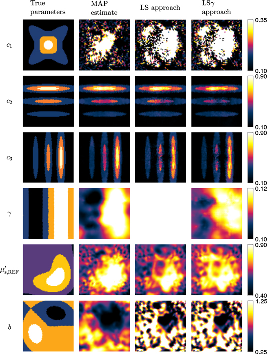
Figure 2. True and reconstructed chromophore concentrations  ,
,  ,
,  , Grüneisen parameter γ, and scattering parameters
  and b for the case of sharply varying material parameters. First column shows the true parameters. Second column shows the MAP estimates. Third and fourth columns show the estimates using the LS and LSγ approaches respectively.
Download figure:
Standard image High-resolution imageTable 1.
Absorption spectra used in this paper:  corresponds to fat [53],
  and
and  to oxygenated and deoxygenated blood [54].
 (nm) (nm) |
 ( ( ) ) 
|

|

|
|---|---|---|---|
| 700 | 0.0700 | 0.9781 | 0.1713 |
| 800 | 0.0750 | 0.4496 | 0.4632 |
| 900 | 0.0800 | 0.4754 | 0.7155 |
The computational domain  was composed of 9016 triangular elements and 4629 nodes. After simulating the noiseless data
  , it was interpolated onto an inversion grid composed of 5022 triangular elements and Q = 2598 nodes. The interpolation was performed in order to avoid the inverse crime. Additive error with a Gaussian white noise distribution was added to the noiseless data such that
  . It was drawn from a distribution with
  , with
  ,
,  being a vector of zeros and
  being the identity matrix.
4.2. Reconstructions
The MAP estimates were obtained by minimizing (12) as described in section 3. The parameters of the combined prior  were
were
where  indicates a block diagonal matrix formed with the matrices in the braces, and the parameters correspond to priors of the estimated parameters such that
 ,
,  ,
,  ,
,  ,
,  is a vector of ones, and each covariance matrix of the priors has the form

where  is given by (13), and
  are scaling parameters for the marginal priors. Values used for the prior means
  and the scaling parameters
  are given in table 2. The prior parameters were chosen by presuming good quantitative prior information of the form
  , and
, and  , where w is the true γ,
  , or b. Parameters
  and
and  were chosen similarly, but assuming that
  and
and  . Correlation length of
  was used in computing
  .
.
Table 2. Prior parameters used for the MAP estimate.
| w |

|

|
|---|---|---|
| c | 0.5000 | 0.2500 |
| γ | 0.1100 | 0.0001 |

|

|

|
| b | 0.7500 | 0.2500 |
For the noise statistics, a distribution of  was used in the inversion, with accurately defined mean and covariance
The second column of figure 1 shows MAP estimates obtained with (12) for the case of smoothly varying spectral parameters. The estimate of  is clearly worse than the estimates of the other chromophore concentrations
  and
and  . This is due to the low absorption spectrum of the first chromophore in comparison to the other two, as evident from the values listed in table 1. The main contributors to the optical absorption in the domain are the oxygenated and deoxygenated components of blood, with concentrations
  and
and  . Their reconstructions are comparable in visual quality to each other, and their shape resembles that of the true parameters. The Grüneisen parameter γ and the reduced scattering parameters
  and b are in their overall shape similar to the true parameters, but show more distortion in comparison to
  and
and  .
.
The second column of figure 2 shows MAP estimates in the case of sharply varying spectral parameters. The reconstructions are similar to the case of smoothly varying spectral parameters. Estimates of  and
and  show the sharp changes in the true parameters. However, the estimates of
  , γ,
, γ,  and b do not show the sharp changes, while the overall shape of the estimates are similar to the true parameters.
4.3. Reference reconstructions
For a comparison with the direct estimation of the spectral parameters, the same parameters were estimated indirectly, and more conventionally, by first estimating the optical coefficients at each wavelength. A Bayesian approach [37] was used to obtain the optical coefficient estimates, then the spectral parameters were fitted to the estimated absorption and scattering parameters based on (3). The approach was performed under two conditions: with a known and unknown γ. These are referred to as LS and LSγ approaches for the known and unknown γ respectively. The approaches were performed for the smoothly and sharply varying material parameter cases.
Both in the case of known and unknown γ, the prior parameters for the absorption and scattering in the LS and LSγ approaches were defined similarly as in section 4.2 as  and
and  with
with  and
and  with w being either
  or
or  . The prior parameters of
  and
and  were different for each of the investigated wavelengths. In the LSγ approach, where γ was assumed to be unknown, its prior was defined as
  where
where  and
and  . Values of the prior parameters are shown in table 3. As in section 4.2, accurate mean and covariance were used for the additive error in both of the approaches.
Table 3. Prior parameters used for LS and LSγ approaches.
| w |

|

|
|---|---|---|

|
||

|

|

|

|

|

|

|
||

|

|

|

|

|

|

|
||

|

|

|

|

|

|
| γ | 0.1100 | 0.0001 |
The estimates of  and
and  were computed at the three wavelengths using the true value of γ in the LS approach. For LS γ approach γ was estimated as well. Following the estimation of the absorption and scattering using the LS and LSγ approaches, the spectral parameter model (3) was fitted to the estimates using a least squares method.
The third column of figure 1 shows the estimates of the spectral properties of the target for the LS approach (known γ) for the smoothly varying parameter case. It is observed that the estimates of  and b do not resemble the true parameter distributions, while the estimates of
  ,
,  and
and  do. Similar behaviour is observed in the case of sharply varying material parameters shown in the third column of figure 2.
The fourth column of figure 1 shows the estimated spectral parameters of the target for the LSγ approach (unknown γ) for the smoothly varying parameter case. The estimates of  and
and  seem to resemble the true parameters. It is oberserved that the estimate of γ is not very good and that the estimate of
  is worse than in the LS approach. As in the LS approach, the estimate of b using the LSγ does not resemble the true parameter distribution. The fourth column of figure 2 shows the estimates for the sharply varying material parameter case. In this case
  resembles the true parameter distribution even less than in the case of smoothly varying material parameters. Otherwise the estimates behave as in the case of the smooth material parameters.
4.4. Comparison of the reconstructions
The relative error of the estimated spectral parameters was computed using

where h is the true parameter and  is the estimate. Table 4 shows the relative errors of the MAP estimates and the estimates obtained with the LS and LSγ approaches. The relative errors are shown for the smoothly and sharply varying parameter cases. Based on the relative errors it is observed that the direct estimation of the spectral parameters results in better estimates than by first estimating the optical parameters at each wavelength separately and then fitting the spectral parameters based on the spectral parameter model. Estimates of
  with the LS approach (known γ assumption) were better than when using the MAP estimate. However, this assumption is not usually valid as the Grüneisen parameter is typically unknown.
Table 4. Relative errors of the estimates in percentage for the smoothly and sharply varying parameter cases. Relative error shown for the MAP estimate, as well as for the LS and LSγ approaches.
| Smooth parameter case | Sharp parameter case | |||||
|---|---|---|---|---|---|---|
| MAP | LS | LSγ | MAP | LS | LSγ | |

|
91.8 | 331.0 | 442.1 | 86.8 | 345.0 | 386.5 |

|
6.5 | 15.1 | 17.1 | 8.3 | 13.7 | 19.7 |

|
7.9 | 17.4 | 21.4 | 11.8 | 21.4 | 26.3 |
| γ | 2.9 | 4.9 | 4.4 | 5.0 | ||

|
9.4 | 7.7 | 12.8 | 12.6 | 8.7 | 13.7 |
| b | 17.3 | 61.0 | 69.2 | 25.2 | 58.4 | 56.8 |
5. Discussion
In this work a Bayesian approach to SQPAT was described. It employed generic and widely-used spectral tissue models, and was tested in two problems, each composed of three different chromophores with biologically relevant tissue parameters. The first problem had spatially smoothly varying spectral parameters, while the second had sharp changes. In both cases all the parameters (three chromophore concentrations, Grüneisen parameter, and two scattering parameters from Mie scattering theory) were reconstructed to good accuracy from the simulated measurement data formed with six measurement composed of two illuminations at three different wavelengths.
The superiority of the direct estimation of the spectral parameters was demonstrated numerically, by comparing the estimates to ones obtained by first estimating the absorption, scattering and the Grüneisen parameters separately at the three wavelengths and then fitting the spectral parameter model to these estimates. The latter approach failed to provide as accurate estimates as the direct estimation of the spectral parameters.
The approach presented allows the inclusions of quantitative prior information of the estimated parameters into the reconstruction. In addition, although not investigated in this paper, this approach also makes it possible to include information regarding the noise statistics in the reconstruction, as in [37]. As the inverse problem in SQPAT is two-fold, any error in the initial pressure distribution estimate (formed from the noisy measured transient ultrasonic waves) is certain to affect the estimates obtained in the optical inverse problem. The error in the initial pressure distribution estimate might have a nondiagonal and spatially nonuniform distribution in terms of its covariance structure, when it is modeled as a random normally distributed noise process. This could be a consequence of nonideal measurements of the acoustic signal, for example, limited view measurement on the boundary, large area transducers causing averaging of the received signal, or band-limited response of the transducer. The error could also be a consequence of neglecting acoustic inhomogeneities in the investigated target, or using approximative reconstruction algorithms to obtain the initial pressure distribution estimate. The error might be of numerical source by nature as well. An example of such could arise from errors caused by insufficient discretization in the numerical estimation of the intial pressure distribution. Utilizing the Bayesian approach should allow compensation of the said types of imperfections.
For this investigation, the DA was used as the model for light propagation in tissues. A more accurate model for the situation, considering the size of the domain and the values of absorption and scattering, is the RTE [46, 47]. However, practice has shown that the DA works as well in QPAT, at least when the main interest is the optical absorption parameter [35, 38, 40, 42, 55]. This is probably due to the nature of the data in QPAT as it is more sensitive to the absorption, than it is to the scattering [26]. Therefore, it was chosen as the light transport model for this work. In the future, this same approach will be tested using the RTE. Furthermore, compensating the modelling error caused by using the DA with respect to RTE through Bayesian approximation error modelling could be considered, as in [56].
Extension of the presented approach from two dimensions to three is not without issues. As the number of spatial dimensions increases, so does the total number of discretization points involved in the computation. This means that the size of the covariance matrices in the computation and the simulation time of the forward model increase as well. These factors will make the reconstructions slower and more memory demanding in three dimensions. In this work, the time to compute the estimates of the spectral parameters using the approach presented was around 31 min using MATLAB (R2011b, The Mathworks) code on a workstation with two Intel Xeon E5649 processors.
Acknowledgments
This work has been supported by the Academy of Finland (projects 136220, 140984, 272803, and 250215 Finnish Centre of Excellence in Inverse Problems Research) and by the strategic funding of the University of Eastern Finland.
Appendix A.: Finite element approximation of the forward model
Variational form of (2) is

where  is a test function. Approximating κ,
  , s and
  as sum of linear basis functions
  (n = i or q)
and inserting (A.2) into (A.1) with choice  for the test function results in the discretized form
Note that  in (A.3). Though s only needs to be defined on the boundary
  , in the above it is defined in the entire domain
  for convenience. Defining matrices
  by their value in pth row and qth column, and vertical vector
  by its value in the pth row as
equation (A.3) can be expressed in matrix notation

where
A finite element approximation of fluence  can readily be obtained from (A.5) with matrix inversion, from which an approximation of the initial pressure distribution (1) is obtained as

Defining  (
( ),
), 
 ,
,  and
and  , and substituting
  and
and  with their discrete spectral representatations at wavelength λ
in (A.7) results in

where
Forward models (5) and (6) follow from (A.9)–(A.10) by replacing λ and s with  ,
,  , and defining
  .
.


