
Abstract
We consider whether it is possible to recover the three dimensional strain field tomographically from neutron and x-ray diffraction data for polycrystalline materials. We show that the distribution of strain transverse to a ray cannot be deduced from one diffraction pattern accumulated along that path, but that a certain moment of that data corresponds to the transverse ray transform of the strain tensor and so may be recovered by inverting that transform given sufficient data. We show that the whole strain tensor can be reconstructed from diffraction data measured using rotations about six directions that do not lie on a projective conic. In addition we give an inversion formula for complete data for the transverse ray transform. We also show that Bragg edge transmission data, which has been suggested for strain tomography with polychromatic data, cannot provide the strain distribution within the material but only the average along the ray path.
Export citation and abstract BibTeX RIS

Content from this work may be used under the terms of the Creative Commons Attribution 3.0 licence. Any further distribution of this work must maintain attribution to the author(s) and the title of the work, journal citation and DOI.
1. Introduction
This paper examines whether it is possible to recover the three dimensional strain tensor field tomographically from neutron and x-ray diffraction data for polycrystalline materials.
The tomography of symmetric rank two tensor fields defined on domains in  is well studied, in particular comprehensive results are presented in [18]. So far these results have not been extensively used in practice. Of course any attempt to recover the six independent spatially varying components of a tensor field will inevitably demand the collection of a large quantity of data, and the necessary computational resources are required for its inversion. As the computational challenges fall to the advance of Moore's law experimentalists are revisiting the requirements for data collection. In the case of polarized light tomography for the study of strain in transparent photoelastic objects systems already exist [3, 21, 24] and indeed there are explicit analytical [10] as well as numerical [20], reconstruction algorithms for the Truncated Transverse Ray transform, which describes that system for sufficiently small strains.
Recent interest has been shown in accurate non-destructive high resolution measurement of strain in polycrystalline materials. Traditionally strain fields are mapped in one, two or three dimensions by defining a gauge volume by slits or collimators that is then translated step by step in one two or three dimensions to recover a map of a strain component (figures 1, a, b). One disadvantage of this method is that it is time consuming while for synchrotron diffraction, at least, the gauge is often much longer along the transmitted raypath than lateral to it (figures 1, a, b) thereby limiting the spatial resolution (see [23]). Korsunsky et al point out [8, 9] that if strain tomography were possible then this would enable the reconstruction of the strain field across slices or volumes in three dimensions potentially alleviating both of these issues.
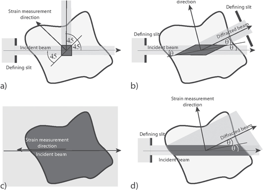
Figure 1. Schematic showing the geometry for the point wise measurement of strain by (a) neutron diffraction at the characteristic 90 scattering configuration, (b) high energy synchrotron diffraction and strain radiography using (c) Bragg edge neutron diffraction and (d) low scattering angle synchrotron diffraction. In each case the gauge volume is shaded dark grey.
Download figure:
Standard image High-resolution imageHere our aim is to take a fundamental look at the potential for strain tomography from a mathematical viewpoint, to examine what information can be recovered and to identify how best to extract information about strain from the information accumulated by a ray. In particular we will show that the average of the transversal component of the strain tensor along a ray is related to a moment of superimposed, distorted Debye–Scherrer rings that can be measured in the experiment. We propose a reconstruction of this component from moment data available for all rays orthogonal to a chosen direction. For six suitably chosen directions the strain tensor can be uniquely recovered and we give a simple criterion to test if the directions are suitable. We also give a reconstruction algorithm assuming complete data. We see that the method of [8] is essentially correct except they use a different average over the Debye–Scherrer ring.
By contrast, we show that at least in its simplest interpretation, Bragg edge neutron diffraction tomography for polychromatic beams [1, 2, 4, 15–17, 22] can only measure the change in path length of the beam through the material (i.e. the average through thickness strain) and is unaffected by the distribution of strain and so strain cannot be simply tomographically reconstructed using Bragg edges.
2. Ray transforms of rank 2 tensor fields
Let  be the space of smooth compactly supported functions on
  with values in the six dimensional vector space
  of symmetric two-tensors on
  . The simplest ray transform we can take is to apply the scalar ray transform to each component

where  . Without loss of generality, when describing the ray
  , we can take ξ to be a unit vector and
  . Following Sharafutdinov [18] we also define the transverse ray transform

where

is the projection on to the plane  , we identify rank two tensors with matrices for the purposes of multiplication and
  is the identity matrix.
We also define the longitudinal ray transform 

While we have formulated these transforms on compactly supported tensor fields it is equally possible to extend them to the Schwartz space of test functions, and to distributions for example using the formal adjoint as is done for X in [14]. It is also simple to show that, like X, J and I are bounded maps between suitable Sobolev spaces, see for example [20].
3. Determination of a symmetric matrix from its quadratic form
Our integral transforms of tensor fields will often enable us to recover a diagonal component in some frame at each point. With this in mind we notice that a symmetric matrix  determines a quadratic form
  and it is well known that the off-diagonal elements of A can be determined from Q using the polarization identity

Here Q evaluated on the unit basis vectors  as well as the vectors
  and
and  , but more generally it is convenient to have geometric criteria that six non-zero vector xi,
  are sufficient for
  to uniquely determine A. Of course one can simply say that the expressions

are independent as linear forms in the aij, or equivalently that the outer products  span
span  , but it is useful to have a geometric rather than algebraic criterion. Notice that if the equations are not independent there must be some non-zero symmetric matrix A in the null space of the linear operator defined by (6), with
  for all
  . This is precisely the same as saying that the six points on the projective plane P2 lie on a projective conic defined by (non-zero scalar multiples of) A. Indeed any five distinct points in P2 lie on a unique projective conic so what is needed is a criterion to tell if the sixth point lies on the conic defined by the other five. We have exactly what we need in the classical Pascal's theorem (see figure 2) and its converse, from projective geometry. Recall that the projective plane can be considered as simply the unit sphere
  under the identification
  , hence points on P2 are simply directions in
  . Projective lines in P2 are the pairs of antipodal points lying on the intersection of a plane through the origin with the unit sphere. We now have Pascal's theorem and its converse [5].
Theorem 3.1. Six distinct points ABCDEF in the projective plane lie on a conic if and only if points of intersection of the lines AB with DE, CD with AF, and BC with FE are colinear.
One important special case is where the six directions xi lie on some antipodal pair of small circles defined by  for some fixed unit vector k and
  . Such points do lie on a projective conic and so A is not determined by the
  . On the other hand given five distinct points on such a pair or circles and a sixth that does not, A is determined by the
4. x-ray diffraction and strain
A crystal consists of a periodic spatial arrangement of atoms (which we take to be located at points). For our purpose the important feature is that there is a family of planes1
normal to a set of one of more unit vectors2
ki, separated by a distances di. It is usual to call each family of parallel planes a crystallographic plane, thought of as representative of the equivalence class. When a parallel beam of monochromatic x-rays, with wavelength λ, in direction ξ are incident on the crystal such that  satisfies Bragg's law (see figure 3),

for some  , part of the beam is diffracted and continues in the direction η in the plane defined by ki and ξ and at an angle
  to ξ. The integer n is called the order of diffraction and we will denote
  by
by  . In vectors

Note that ki is defined only up to sign but the choice of sign does not effect η.
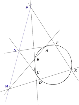
Figure 2. The classical Pascal theorem is explained using a hexagon joining the six points ABCDEF. The opposite sides of the hexagon are extended and meet at co-linear points PMN
Download figure:
Standard image High-resolution image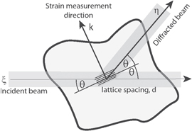
Figure 3. Bragg diffraction from one crystallographic plane
Download figure:
Standard image High-resolution imageIn practice one might expect to observe diffraction from between one and three orders, and  . Bragg diffraction is thought of as elastic scattering in that the diffracted x-rays have the same wavelength (and hence energy) as the incident x-rays. It is also described as coherent scattering as phase relationships are maintained on the length scale of the distance between planes. We will ignore any attenuation of the diffracted x-rays by the material.
A polycrystalline material is understood to be a bounded region  and a finite set of subsets
  (crystals) each with a positive measure and a Lipschitz boundary such
  and their pair-wise intersection is measure zero. Each of the
  is a crystal with the same set of planes and distances between planes except that the normals to the planes are rotated by some element of the rotation group
  relative to some reference configuration. Metals form typical examples of such polycrystalline materials and in this case the
  are called grains and we are assuming the grains all have the same crystal structure and there are no gaps between them. We note also that is an idealisation. For example real crystals can have defects and impurities where the periodic structure breaks down, they might have residual stress that distorts the crystal structure, and except at absolute zero temperature the atoms in the crystal vibrate about their equilibrium positions.
We now describe the effect of x-ray diffraction on our sample of polycrystalline material. We will assume that the x-rays incident on D form a narrow beam (for example cylindrical) centred on some ray. This is possible for example using a synchrotron source. We will assume that the width of the beam is sufficient that its cross section includes a large number of crystals across the width of the beam. On the other hand the crystals themselves consist of sufficiently many planes for well defined Bragg diffraction from one or more planes. We are of course considering the beam to consist of plane waves propagating in a given direction and yet confined to a beam (collimated). This standard ray optics approximation is justified as the wavelength of x-rays is similar to the spacing of the atoms, and we have many crystals, let alone atoms, in the width of the beam.
Let us now assume that we are observing the transmitted and diffracted x-rays where they are incident on a screen normal to the incident direction ξ, at a distance large compared to the size of D. Although clearly it is important for constructive interference between x-rays on the scale of the distance between crystallographic planes, x-rays from our synchrotron will not be coherent over the path length between the sample and detector. Consequently the detector will measure the sum of the squared magnitude of all the x-ray waves incident at that point, or more realistically over a small square pixel containing that point.
For a beam along a given ray  the diffracted rays when observed at a distance L on a plane normal to the ray lie on circle centred on the projection of x on to this plane with a radius
  , for the i the crystallographic plane and the n the order diffraction. The intensity of the observed ray in a circle
  is the measure of the intersection of the beam and the crystals
  such that
  results in a diffracted beam at y on the plane, that is

where

Of course as we have described the situation this will result in a delta function measure for each of the finite number of crystals, but in practice for sufficiently fine crystals with orientations uniformly distributed in  what is observed are circles of uniform intensity around the ring, and we must regard this as a limiting case of infinitely many crystals. Also in practice one does not observe a delta measure on the circle but some distribution of intensities with the maximum on the circles. This is due to the various approximations we have made including the distance L being finite.
We now consider the effect of elastic deformation on the material. Mathematically this means that we have a diffeomorphism  that takes the unstrained to the strained material. Of course the intersections of the crystallographyic planes are also preserved by this deformation. Under the usual small strain assumption we write
  for some small vector field U. We will assume that the crystals are sufficiently small that
  can be taken to be constant over a crystal for the purposes of studying the diffraction.
We now consider the effect of the deformation on the separation d of the planes normal to k in one crystal. Let  , where
  is the derivative of F, be the deformed separation vector we have


where  is the infinitesimal strain tensor. Hence we have the relative change in d

By contrast  so to the leading order term the direction is unchanged. We see that the circles in the diffraction pattern of the unstrained case, Debye–Scherrer rings, are distorted by the strain. Let
  with
with  the unit vector in
  in the plane of k and ξ then

Often for high energy, small λ, x-rays (called hard x-rays) and low orders n the Bragg angles  are small, perhaps two or three degrees. On the other hand it is possible in a synchrotron beam to have the the detector screen many meters away. This means that while the Debye–Scherrer rings can still be measured the normal to the plane ki, giving rise to the diffraction can be considered approximately parallel to the screen. This gives rise to a the deformed Debye–Scherrer ring being simply an ellipse defined by the points
  such that

or with the small strain approximation.

and using the small θ approximation in k we have approximatly

where  is the radius of the unstrained Debye–Scherrer ring for the crystallographic plane ki and order n. This describes the situation for uniform strain. The diffraction pattern observed will be the superposition of (slightly blurred) ellipses, and any given point on the detector plane will include x-rays diffracted from points along the line with different strains that meet the Bragg condition.
5. Extracting information from the diffraction pattern
We will consider the case for small θ, in which the diffraction pattern contains only information about the strain transverse to ξ,  . We might consider this a case of rich tomography in that for each ray we have not a scalar or a vector value but a function of two variables. One approach would be simply to solve the linear equations relating the strains in a grid of voxels to the intensities measured on the screens. Even for only one rotation axis, for similar pixel and voxel dimensions, we would have far more equations than variables and solving such a system would be inefficient. Our aim therefore is reducing the redundancy of the data while still retaining sufficient information for a unique reconstruction.
Given the wealth of data in a complete diffraction pattern it might be supposed that we could at least reconstruct the distribution of strains along the x-ray beam. A typical diffraction pattern from a small area with uniform stress consists of a series concentric ellipses for different orders. For a complete beam path we have the sum of such ellipses weighted by the prevalence of each transverse strain along the beam path. We might suspect that we could fit a weighted sum of ellipses to this pattern and then interpret the weights of the proportion of each transverse strain tensor present along the ray. We will show however that this is not the case as different distributions of ellipses can produce the same image.
An ellipse centred at the origin in the plane can in general be represented as a symmetric 2 × 2 matrix A with the points on the ellipse satisfying  . In our case A(s) is the matrix

in a suitable basis on 
The unit density on the ellipse is therefore the delta measure

we use the notation  for the unit measure on a set S and just δ for the standard Dirac delta measure at the origin in one dimensional space, that is an abbreviation for
  . Ignoring the spread of the of the Debye–Scherrer ring our diffraction pattern is the sum of such densities as A runs over the A(s) be represented (in this idealized case) by

where we have suppressed x and ξ as for the present discussion we regard them as fixed. We seek then information about the distribution g(A) of A that gave rise to this. In a very general sense (see for example [6, 12]) a Funk–Radon transform is the integral of a function on the plane over a two parameter family of curves. In this respect the two dimensional Radon transform (the integral over all lines) and its adjoint, also known as the backprojection operator, (the integral over translated sine waves of the same frequency over half a period) are both Funk–Radon transforms.
When straight lines occur in a photograph one way to detect them automatically is to take a filtered Radon transform, known as the Hough transform in computer vision, as lines densities in the image are mapped to delta functions by the radon transform. The Hough transform has been generalized to the detection of ellipses in a photograph [25] and one might expect that this would work for x-ray diffraction of polycrystalline materials. However the family of concentric ellipses is parameterized by three variables  and a22, which satisfy
  and
and  to ensure the matrix is positive definite. Alternatively the semi-major axes and the rotation of the principal axis can be used as three parameters.
Consider polar coordinates  which transforms
  to
to

which is the equation of a plane in  space normal to the vector
  and a distance
  from the origin. As r varies for fixed ψ this gives us a family of parallel planes, while as ψ varies the
  describes a circle in the plane
  . Our diffraction data is thus a two parameter family of plane integrals and is insufficient to determine a general density in the three dimensional
  space. If the set of possible densities were sufficiently restricted it may well be possible to recover it from integrals over a two parameter family of curves. We could assume that it is concentrated on a (possibly self intersecting) curve as in our case it is parameterized by s, but as this curve is unknown this is of no obvious help. See figure 4.
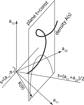
Figure 4. The space  illustrating that the distribution of A values along one beam will cluster around a curve.
Download figure:
Standard image High-resolution imageThe case in which  for t a known constant has a unique solution as our planes intersect this plane in all possible lines, in fact this is exactly the two dimensional Radon transform in the variables
  where
where  . However the determination of the distribution of the perpendicular strain along a ray from one diffraction pattern (for one energy of x-ray) is clearly too ambitious in general. Indeed, even in special cases where it is possible it only gives the information on which plane strains tensors arise and how frequently, not where they are on the line.
Instead we set a more modest aim: to determine the centre of mass in of the distribution in  space. This we can do from only three choices of direction
  as we will show.
6. Average strain from moments
Korsunsky [8] assumes that the average strain along a ray in a given direction normal to the ray is proportional the deflection of the diffraction pattern and the intuition behind this is sound, but as the diffraction pattern is an average of elliptical Debye–Scherrer rings and each of those rings is itself blurred it is not clear what average value for deflection should be taken. In this section we show that a certain moment of the diffraction pattern in the required direction is the correct choice.
We have in general

We have used the measure  as it is the measure associated with the Fröbenius norm on
  and hence invariant under the action of
  .
.
Without loss of generality we now take  so that
  and (23) becomes


We now define the moment of  in the direction of any y as
As the substitution  in (24) gives
  .
.

noting that as A is positive definite  . Applying a rotation of coordinates we see that for a general unit vector y

in particular (27) applies with 2 in place of 1.
The defining property of the density g guarantees

so we have from these three moment calculations along radial directions of the diffraction pattern the transverse ray transform  .
.
7. Measurement and reconstruction
For the transverse ray transform J a simple explicit reconstruction method is suggested by [18]. Let ζ be any unit vector and consider any  . We then have

as the projection leaves ζ unchanged. We note this is exactly the two dimensional Radon transform of the scalar  in the plane through x normal to ζ. Taking ζ as each of the unit basis vectors ei in turn we can recover the diagonal terms
  by Radon transform inversion plane by plane. Experimentally we would achieve this by rotating the object half a turn about each the coordinate axes. To obtain the off diagonal terms (again a special case of the polarization identity(5) note that the choice
  gives
gives

hence we obtain the off diagonal term  by a further rotation about this tilted axis, and the other off diagonal terms are obtained similarly. In general any six vectors
  chosen according to the criterion in section 3 will yield sufficient data. We now have
- 1.For any plane π normal to a unit vector ζ the components of
 can be obtained as the inverse Radon transform of the moment data for the diffraction patterns for the rays in π.
 - 2.Given six unit vectors that do not all lie on the same projective conic, the moment data for all the rays with and with non empty intersection with D determine and hence six linear equations for known can be solved to give
 everywhere in D.


While this method gives a proof sufficiency of data, one suspects that a reconstruction would be possible with less than six rotation axes. Indeed for each ray the above algorithm uses a moment of the diffraction pattern only in the direction of the rotation, a single measurement of a one-dimensional section of the diffraction pattern. It would be desirable for practical purposes to have an explicit reconstruction algorithm that uses rotation about fewer axes, but makes better use of the data for each ray. We do not currently have such an algorithm, but of course one could take a brute force approach by solving a very large sparse system by an iterative method from numerical linear algebra. At the other extreme, in the next section, we give a reconstruction formula using data from all rays.
8. Inversion of the transverse ray transform with complete data
For the scalar x-ray transform there is an explicit inversion formula [11] for data for all rays passing through the support of the function to be recovered. This formula is a generalization of the filtered back projection formula for the two dimensional case, and it has several uses even though it is not usually practical to measure over a set of rays forming a reasonably uniform sample of all the four dimensional space of possible rays. For example if one can measure an open set in the space of rays, by tilting a sample about two axes in a parallel beam with a planar detector, one can show that the inverse ray transform has a unique solution using the Paley–Weiner theorem and analytic continuation. Of course this reconstruction is unstable in any Sobolev spaces [7] but it can be analysed using microlocal methods to understand the artefacts that result from such a truncated data reconstruction. In anticipation that similar limited data may be available for x-ray diffraction we derive an explicit filtered back projection inversion formula for the transverse ray transform, following closely the method used in [18] for the Truncated Transverse Ray transform. This section and the one that follows uses several concepts from the general theory in that book and is not needed for the understanding of the simple reconstruction procedure detailed in the previous section.
First some essential notation. We will denote by  the backprojection operator

where Ω is the unit sphere and ω its standard measure. On  , the space of smooth symmetric rank k tensors fields we denote by
  the generalization of divergence

(we use the convention of summation over repeated indices) and the negative of its formal adjoint, the symmetric derivative 
where σ is the symmetrization operator on tensors. We will denote by Δ the Laplacian taken on components. The inverse  is defined by convolution with the fundamental solution. The trace of a rank 2 tensor field f is denoted by
  .
.
We are now ready to state explicit inversion formulae using complete data for the transverse ray transform
Theorem 8.1. Let  be a symmetric tensor field then

9. Sketch of proof of theorem 8.1
We begin with some formulae for the Fourier transforms of terms that arise in the operators BJ which are simplifications of those given in [Sec 2.11, 18] for the specific cases we need. For m = 0,1, or 2 define  by
by

Using symmetry in t and the substition  we obtain


For m = 0 this is just the classical result giving the inverse of the scalar ray transform in three dimensions:  . For example in [11] equation (2.2) on p19 with
  , indeed we have immediately

and using Eq (2.11.6) of [18] we have also for f a vector field

For m = 2 we need the linear operator

which is  contracted with f over two indices. To see this notice that in components this is a sum of terms of the form
  over all permutations π of four symbols. Of the 24 permutations 16 give indecies i1 and i2 on separate factors Π whereas 8 result in i1 and i2 on the same factor. In [18]
  is denoted by
  . We have then

To apply these results to the transverse ray transform first we expand equation 3 as
Now we write

corresponding to the three terms in equation 44. We notice G1 is simply BX and hence

and the third term is exactly  so
so

For the second term one must look again at equation 37 for m = 1, but applied to  . We find

Taking the Fourier transforms of these expressions gives us the following lemma:


We now wish to invert these expressions to obtain thm 8.1. First we write
 and use
  and
and
Substitution of (50) in (49) gives

We now verify by direct substitution that

theorem 8.1 now follows from the definitions of d and δ. Such calculations are simplified by the observation that the algebra generated by the five terms in the brackets in (35) is finite dimensional over the field generated by δ. This means for elements that are units one has to find only five coefficients to compute an inverse.
We note that the pseudo differential operator in theorem 8.1 is elliptic as it has an explicit (left and right) inverse for all  . This means that micro-local methods, such as Lambda Tomography, may be used to recover some of the singular support of a non-smooth from limited data in a straightforward extension of the method used for the scalar x-ray transform [13]. Indeed the operator
  is simply the inverse of the scalar x-ray transform applied to each component. This means that any limited data inversion method for the x-ray transform, for example methods for lines passing through a curve external to the support, yields a reconstruction algorithm for J.
10. Insufficiency in Bragg edge tomography
In the approach we have described so far for each ray the data observed is the diffraction pattern. Another approach, suggested for neutron strain tomography, is apply polychromatic beam containing an interval of wavelengths λ at known intensities and use a single detector for that ray that can resolve the spectrum–the energy transmitted at each frequency. The decrease in the transmitted energy is due to the diffraction of the neutrons. For a fixed ray, wavelength, order and crystallographic plane some neutrons will be scattered when there is a θ in  such that
  given that there is a sufficient range of distorted distances d'. What is observed [17] is that the transmitted energy against λ curve has a discontinuity, a sudden increase, as theta approaches
  , so the neutrons are 'back scattered', and no further diffraction happens from that plane and order. This discontinuity is termed the Bragg edge. The treatment in the literature [2, 15–17, 19] is quite heuristic and the various curve fitting procedures to quantify the mean of
  along the line
  . However for our purposes what matters is that the measurements give only

An important distinction between J and I is that even for complete data I has a null space consisting of f such that f = dh for some smooth vector field h. We will need to treat the case where f is zero outside D so has a discontinuity on  so we will give an explicit argument. In particular we note that in the interior
  . For simplicity take
  and assume D is convex


where  and
and  are the x3 coordinates of the intersection of the ray with
  . We see that such a technique is only sensitive to the overall change in thickness of the sample along the ray and not the distribution of strains. The restriction to a convex body is of course unnecessary, we would simply get the sum of the thickness change in each component of the intersection of the ray with D. In the case of a void within an object with known boundary this may well be useful as the displacement of the void could be be measured more accurately using Bragg edge than conventional tomographic methods.
11. Conclusions
In conclusion we see that it is indeed possible to obtain the component of the strain normal to a plane from observing the diffraction due to a narrow beams in that plane. We recommend that rather than using a curve fitting procedure the appropriate radial moment of the diffraction profile is used. If six well chosen rotation axes are used and for each axis such diffraction measurements are made for a set of lines in the plane, then all six components of the strain can be reconstructed at points on the intersection six of these planes. To reconstruct the stress throughout the sample this way requires a time consuming measurement process. It remains to be seen if there are explicit reconstruction procedures using more of the diffraction data for fewer rotation axes. Certainly it would be possible to construct a system of sparse linear equations for a discretization of the problem and attempt a solution using standard iterative algorithms.
We have also shown, contrary to previous assertions, it is not possible to simply reconstruct the internal strain distribution within a body from Bragg edge measurements without some form of extra information because it just gives the average fractional change in dimension (strain) along the ray path.
Acknowledgments
This work was partly funded by the EPSRC building global engagements grant MIRAN (EP/K00428X/1), the Tomography CCPi (EP/J010456/1), the Next Generation Multi-Dimensional x-ray Imaging grant (EP/M010619/1), the Residual Stress & Damage Characterization Extending Across. Length and Time Scales grant (EP/F028431/1), the Structural evolution across multiple time and length scales grant (EP I02249X/1) and the authors are grateful for the helpful discussions on this topic with Vladimir Sharafutdinov while visiting under the MIRAN programme. The authors would like to thank Alexander Korsunsky and Brian Abbey for helpful discussions and for feedback on earlier drafts, and the anonymous referees for their suggested improvements. WL would also like to thank the Otto Mønstead foundation for funding the visiting professorship at the Danish Technical University during which the paper was completed.
Footnotes
- 1
In crystallography the planes are indexed by triples of integers called Miller indices but we shall take them to have been enumerated by a single index.
- 2
There are many clashes of notation between crystallography and tensor tomography. In crystallography it is common for our k to be called g and our ξ to be called k