

Abstract
Joint inversion of multiple observation models has important applications in many disciplines including geoscience, image processing and computational biology. One of the methodologies for joint inversion of ill-posed observation equations naturally leads to multi-parameter regularization, which has been intensively studied over the last several years. However, problems such as the choice of multiple regularization parameters remain unsolved. In the present study, we discuss a rather general approach to the regularization of multiple observation models, based on the idea of the linear aggregation of approximations corresponding to different values of the regularization parameters. We show how the well-known linear functional strategy can be used for such an aggregation and prove that the error of a constructive aggregator differs from the ideal error value by a quantity of an order higher than the best guaranteed accuracy from the most trustable observation model. The theoretical analysis is illustrated by numerical experiments with simulated data.
Export citation and abstract BibTeX RIS
1. Introduction
In various application fields, especially in geoscience, one is often provided with several data sets of indirect observations of the same quantity of interest, where each set contains the data measured by different physical principles. For example, when determining the gravity field of the Earth by satellite data we have to combine different types of present or future data, such as satellite-to-satellite tracking (SST) data and satellite gravity gradiometry (SGG) data, as in the case of the GOCE satellite mission [35]. Other examples are related to various problems in geomagnetism, which require a combination of satellite data and ground data at the Earth's surface in order to obtain high resolution models (see e.g. [13]). There is an extensive literature where SST- and SGG-problems were studied and treated separately and independently. For this subject, the readers are referred to the monograph [12] and to the references cited therein.
There is also a closely related research area, where the goal is to jointly reconstruct different underlying modalities from available data under the assumption that the modalities are linked by having structural similarities, such as seismic velocities and density. A generic approach to the joint reconstruction was proposed in [16]. Here, we just mention a very recent publication [11], where the first contribution to the joint reconstruction in multi-modality medical imaging was given. Our study, however, differs from the above mentioned research in its emphasis on the reconstruction of the same modality, such as the gravity potential, from different data sets, such as SST- and SGG-data.
With multiple observation models, such as SST and SGG, each providing approximations of the same quantity of interest, one is left with the choice of which to trust. A more advanced question is what to do with a less trustable approximation, or what is the same, whether the approximation that involves all available observations may actually serve as an effective way to reduce uncertainties in independently inverted models. This question is discussed quite intensively in the geophysical literature, where the term 'joint inversion' was introduced by the authors of [34] for the methods which give the solution of various types of observation equations inverted simultaneously. Similar ideas were also applied in medical applications, e.g. the joint utilization of CT and SPECT observations to improve the accuracy of imaging [4]. A short overview about the application of joint inversion in geophysics may be found in [15], where it was mentioned in particular that there was no standard standpoints using the appellation joint inversion. To distinguish inversion methods based on different data combinations, researchers have introduced different names, e.g. aggregation [31], which was also used in the context of statistical regression analysis [20, 21]. Regardless of their names, what is common across the above mentioned approaches is that they induce stability by simultaneously utilizing different types of indirect observations of the same phenomenon that essentially limits the size of the class of possible solutions [3].
The idea of the joint inversion naturally leads to the methodology of the multi-parameter regularization, which in the present context may be seen as a tool for the compensation of different observations. Multi-parameter regularization of geopotential determination from different types of satellite observations was discussed in [22]. A similar approach was adopted in the high resolution image processing and displayed promising effects in experiments [27]. At this point it is important to note that one should distinguish between multi-parameter schemes, where the regularization parameters penalize the norms of the approximant in different spaces, and the schemes, where the parameters weight the data misfits in different observation spaces. In the former schemes an observation space is fixed, and by changing the regularization parameters we try to find a suitable norm for the solution space, while in the latter schemes the situation is opposite: by changing the parameters we try to construct a common observation space as a weighted direct sum of given spaces. The choice of the regularization parameters for the former schemes has been extensively discussed in the literature. A few selected references are [8–10, 19, 26]. As to the latter schemes (schemes with a fixed solution space), we can indicate only the paper [22], where a heuristic paremeter choice rule is discussed, and the paper [23], where the parameter choice is considered as a learning problem under the assumption that for similar inverse problems a suitable parameter choice has been known. It is clear that such approaches can be used only for particular classes of problems.
Although a simultaneous joint inversion by means of multi-parameter regularization provides acceptable solutions, it still faces methodological difficulties such as the choice of regularization parameters that determine suitable relative weighting between different observations. The goal of the present study is to discuss a rather general approach to the regularization of multiple observation models, which is based on the idea of a linear aggregation of approximations corresponding to different value of the regularization parameters.
This paper is organized as follows. In section 2 we discuss an analog of the Tikhonov–Phillips regularization for multiple observation models. In section 3 we study a linear aggregation of the regularized approximate solutions and its relation to the linear functional strategies [1, 2, 24]. In section 4 we illustrate our theoretical results by numerical experiments. We draw conclusions in the last section.
2. Tikhonov–Phillips joint regularization
In this section, we analyze the methodology from multiple observations to the joint regularization, and lead to the multi-parameter regularization in general form with the SST- and SGG-problems as an incident. Then, different parameter choice schemes in the literature are investigated and which raises the topic of utilizing the diversity of parameter choices. We begin with setting up a general framework.
If m different kinds of observations are assumed, then in an abstract form they enter into determination of the quantity of interest  (e.g. the potential of the gravity or magnetic field), leading to the observation equations

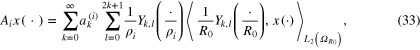
where Ai denotes the design operator, which can be assumed as being a linear compact and injective operator from the solution space  into the observation space
  , and ei denotes the error of the observations, and
  .
.
In a classical deterministic Hilbert space setting,  and
and  are assumed to be Hilbert spaces and

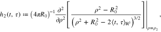
where  is a noise level. In particular, for the spherical framework of the SST-type or the SGG-type problem, the design operators in model (1) have the form

where in case of SST
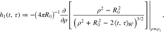
while in case of SGG
and the surface of the Earth  and satellite orbits
  are assumed to be concentric spheres of radii R0 and
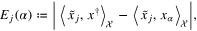
  .
.
The joint regularization of multiple observation models (1), (2) can be formulated as an optimization that involves minimization of an objective functional  , which combines the measures of data misfit
  ,
,  , with a regularization measure. In the spirit of the Tikhonov–Phillips regularization the latter can be chosen as the norm
  of the solution space. In this way, the objective functional can be written as

where  are the regularization parameters. The multiple regularization parameters are introduced in regularization problem (4) to adjust contributions for data misfit from different observation models.
It is convenient to rewrite the objective functional  in (4) in a compact form by introducing a direct sum space of the observation spaces. To this end, for each
  , we use
  to denote the observation space
  equipped with the scaled inner product
  , and define the weighted direct sum
  of the observation spaces
  by
by

where  , and for
  ,
,
By letting  , and
, and  , the objective functional (4) may be represented as

Note that  is a compact linear injective operator from
  to
to  .
.
In the representation (5), we can conveniently obtain the classical Tikhonov–Phillips form of the minimizer  of Φ defined by (4) in terms of
  . Specifically, the minimizer
  of Φ satisfies the equation
where  is the identity operator and
  is the adjoint of
  . Clearly, for any
  the adjoint operator
  has the form
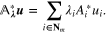
From the representation (5) it follows that the regularized approximant  is the solution of the equation

Equation (6) was obtained in [22] by Bayesian reasoning. It is also suggested in [22] to relate the values of the regularization parameters  with the observation noise levels (variances)
  as follows:

Note that for the given noise levels this relation reduces the multi-parameter regularization (4) to a single parameter one, since only  needs to be chosen.
The heuristic rule (7) can be derived from a bound for the noise propagation error. Specifically, we have that
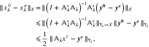
where  . It follows from assumption (2) that
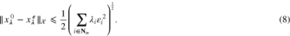
The heuristics behind the rule (7) is clear: the rule equates all the terms from the bound (8) and balances data misfits against each other. Then the final balance may be achieved by making a choice of the last remaining parameter  . The latter can be chosen by known single-parameter choice rules such as the quasi-optimality criterion [33]. We label the above heuristics as 'M1' and provide an algorithm (algorithm 2.1) in pseudo-code to facilitate the usage.
Algorithm 2.1 for M1
Input:
 , where Σ is the parameter set
Output:

1: for j = 1 to
 , where
  do
do
2: for i = 1 to m do
3:

4: end for
5:
 , where
6: if
 then
then
7:

8: end if
9: end for
10:

11: return

There are alternatives to (7), for example, a multiple version of the well-known quasi-optimality criterion [33]. For the sake of clarity we describe it here only for the case of two observation equations (1) (m = 2), which we label as 'M2'. Algorithm 2.2 is provided to illustrate the mechanism behind it. There are also several other ways of selecting the values of the regularization parameters in (4) and (6). In the next section we shall discuss how we can gain from a variety of rules.
Algorithm 2.2 for M2
Input:

Output:

1: for j = 1 to
 , where
  do
do
2: for k = 1 to
 , where
  do
do
3:
 , where
4: if
 then
then
5:

6: end if
7: end for
8: end for
9:

10: return

3. Aggregation by a linear functional strategy
A critical issue in solving the joint inversion problem is the choice of the multiple regularization parameters involved in the model. We may propose various rules for the choice of the weighted parameters of multiple observation spaces if certain a priori solution information is available. In the case of less of dominant criteria, a feasible way to solve the joint inversion problem is to make use of the variety of parameters, or the resulting solution candidates. In this sense choosing a certain linear combination of multiple solutions, which result from different parameter choices, as a new solution to the joint inversion problem may be more efficient. This section is devoted to developing such a method. We propose an 'aggregation' method in a more general sense with the joint inversion problem as a special example. Specifically, we describe the construction of an aggregator and discuss technical difficulties in its realization. We then propose a linear functional strategy to resolve the problem and estimate the related errors. Furthermore, we show that the parameter choice strategy by using the balancing principle can achieve almost the best guaranteed accuracy.
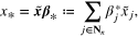
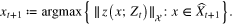
We begin with the review of the aggregation. We assume that there are n various rules available for choosing the multiple parameters  , which result in n different approximations
  ,
,  , to the element of interest
  . In practice, usually we do not know which of these approximations better fits the element
  . Moreover, the approximations
  ,
,  , may complement each other. An attractive way to resolve the arising uncertainty is to 'aggregate' these approximations. That is, we find the best linear combination

in the sense that x* solves the minimization problem
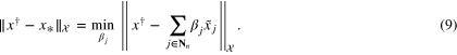
The solution  of (9) is determined by
  , which is the solution of a system of linear equations. To observe this, we need the inner product
  of Hilbert space
  . Letting
and introducing  and
and  , where
  ,
,  , we see that
  solves the linear system

If we assume, without loss of generality, that approximations  ,
,  , are linearly independent, then the Gram matrix
  is positive definite and thus invertible such that

where γ is a constant that depends only on  . Thus,
  has the representation

and
where  .
.
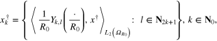
System (10) cannot be solved without knowing the vector  . However, the vector
  involves the unknown solution
  . Therefore, we turn to finding an approximation of system (10). A possible approach is to approximate
  by a
by a  , and to get

by solving the system

This yields an effective aggregator

of  ,
,  . In other words, we find an approximation
  of
of  such that
  is 'nearly as good as' x*. Following this idea, we describe a construction of
  and estimate the resulting errors.
Remark 3.1. In the above discussion, we assume that  are linearly independent. Actually, at the technical level, the more concern would be the degree of their linear correlation, and further, the condition of the Gram matrix
  , which is supposed to be well-conditioned. In principle, one may control this by excluding those members of the family
  that are close to be linearly dependent of others. It is clear that their exclusion does not essentially change the right-hand side of (9). We propose a preconditioning method where we control the condition number of the Gram matrix by utilizing the well-known Gram–Schmidt orthogonalization with a threshold technique.
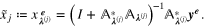
We now describe an iterative scheme for the selection of solutions for aggregation. For  , let
, let  be already selected from Xn to be included in the construction of aggregator (13),
  , and
, and  be the corresponding Gram–Schmidt orthogonalizators, which in addition satisfy

where constants  play roles of the lower and upper thresholds respectively. Consider the next approximant
  and the corresponding Gram–Schmidt orthogonalizator
  . For all
  , we calculate the corresponding Gram–Schmidt orthogonalizator
  by the formula
Denoting by  the set of candidates for
  , we define the selected candidates as follows:
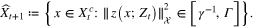
If  , where
  denotes the cardinality of a set A, an additional selection criterion is needed. For example, one may pick
  arbitrarily in
  , or let
If  has been selected,
  can be decided by
  . Let
. Let  . This iterative procedure can be conducted until
  .
.
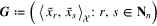
By conducting the above process, we get a selected set Xt from Xn and the corresponding preconditioned set Zt. It is obvious that aggregation among the selected set Xt and among the preconditioned set Zt yield the identical best approximation  in the sense of (9), in view that
  . In the case of aggregation among Zt, the Gram matrix
  becomes a diagonal matrix:
  , where
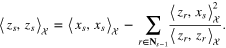
Note that from (14), we have that  , which meets the requirement of (11) with
  . Furthermore, we also get that
  . In this sense, the proposed preconditioning is actually a method of improving the condition number of the Gram matrix.
3.1. Selected results on the linear functional strategy
In this subsection we present an approach to approximate  by using the linear functional strategy as introduced in [1, 2, 24]. The advantage of this strategy is that if one is not interested in completely knowing
  , but instead in only some quantity derived from it, such as the value of a bounded linear functional
  of the solution
  , then this quantity can be estimated more accurately than the solution
  in
in  .
.
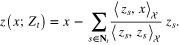
It is reasonable to measure the closeness between an effective aggregator xag and the ideal approximant x* in terms of the accuracy of the best reconstruction of  from the most trustable observation equation

Model (15) is selected from the set of the considered models (1) according to one of the following rules: (a) the operator  makes the corresponding inverse problem less ill-posed than the other design operators, or (b) the data
  are provided with the smallest noise level
  such that

where  is the corresponding observation space
  , for some
  . Then the best guaranteed accuracy of the reconstruction of
  from (15) and (16) can be expressed in terms of the noise level
  and the smoothness of
  . From [29], the smoothness of
  can be represented in the form of the source condition to be described below. According to [29], a function
 ![$\varphi :[0,\parallel A{\parallel }_{\mathcal{X}\to \mathcal{Y}}^{2}]\to [0,\infty )$](https://content.cld.iop.org/journals/0266-5611/31/7/075005/revision1/ip514982ieqn146.gif) is called an index function if it is continuous, strictly increasing and satisfies
is called an index function if it is continuous, strictly increasing and satisfies  . Suppose that an index function φ is given. Let
  be the singular values and the corresponding singular vectors of
  , such that
  , form a standard orthogonal basis in
  . We assume that the following source condition holds

where R is a positive number. It is also known from [18, 30] that
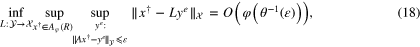
where  for
for  , and the infimum is taken over all possible mappings L from
  to
to  . Clearly, formula (18) ensures that the best guaranteed accuracy of the reconstruction of
  from the observation (15) and (16) has the order of
  .
.
For the purpose of analyzing the Tikhonov–Phillips regularization and its multi-parameter version, such as (4), it is natural to assume that the source condition (17) is generated by a given index function φ that is covered by the qualification, denoted by p, of the Tikhonov–Phillips method (i.e. p = 1) in the sense of [30]. That is to require that the function  , where p = 1 in case of Tikhonov–Phillips regularization, is a nondecreasing function. Then from [30] it is known that the best guaranteed order of accuracy can be achieved within the Tikhonov–Phillips scheme. Recall that for a regularization parameter α, the Tikhonov–Phillips regularization of (15) and (16) is defined as

We recall below a result from [30].
Theorem 3.2. If φ is an index function such that the function  is nondecreasing, then for
Since the Hilbert space  can be identified with its dual, an element
  representing a bounded linear functional
  has certain order of smoothness that can be expressed in terms of the source condition
  with an index function ψ. If we use the Tikhonov–Phillips regularization to approximate the value
  by
by  , then the following result is known (see e.g. [6], remark 2.6 [25]).
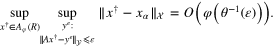
Theorem 3.3. If  and the index functions φ and ψ are such that the functions
  and
and  are nondecreasing, then for
Comparing the above theorems, we conclude that potentially the value of  allows a more accurate estimation than the solution
  , provided that
  satisfies the hypothesis of theorem 3.3. In the next theorem, we show that for the purpose of aggregation the hypothesis of theorem 3.3 is not too restrictive.
Theorem 3.4. If φ is an index function such that the function  is increasing,
  and assume that
  , then for any
  there is an index function ψ such that
  and the functions
  and
and  are nondecreasing.
Proof. Consider the compact linear operator  which is self-adjoint, injective and non-negative. From corollary 2 of [29], it follows that there is a concave index function
  and a constant
  such that
  . Thus,
  admits a representation

where  .
.
Next, we consider the function  and prove that it has the desired properties described in this theorem. It follows from (19) that
  . Moreover, in view of the concavity of the index function
  , we observe that for any

Hence, for  we have that
  and
and
where we have used (20) with  ,
,  and the increasing monotonicity of ω. This proves that the function
  is nondecreasing. The same feature of the function
  may be proved in the same way. Indeed, for any
  we have that
proving the desired result.□
3.2. Application in aggregation
In the framework of the linear functional strategy described earlier, for each  , we can approximate the component
  of the vector
  by
by

where  are feasible substitutes for
  . Combining theorems 3.3 and 3.4, we see that for
  there exists an index function
  such that
  and
and

where  . Theoretically, the order of accuracy
  in approximating
  can be achieved by applying the linear functional strategy with the same value of the regularization parameter α. However, in practice, the function φ describing the smoothness of the unknown solution
  is unknown. As a result, one cannot implement a priori parameter choice
  . In principle, this difficulty may be resolved by use of the so-called Lepskii-type balancing principle, introduced in [6, 14] in the contest of the linear functional strategy. But, a posteriori parameter choice strategy presented in those papers requires the knowledge of the index functions
  describing the smoothness of
  in terms of the source condition
  . This requirement may be restrictive in some applications. The proof of theorem 3.4, for example, gives the formula
  , where both functions
  depend on the unknown index function φ. To overcome this difficulty, we consider below a modification of the balancing principle to achieve the error bounds (22) without requiring the knowledge of φ and
  .
.
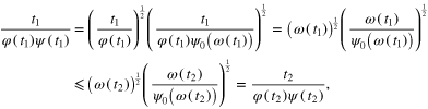
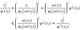
The theory of the balancing principle is known in the literature (see, for example, [14], section 1.1.5 of [25], and [28]). Following the general theory, we formulate a version of the balancing principle suitable for our context. In view of the representation
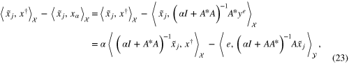
which is well known as the decomposition of the error into the noise-free term and the noise term, we consider the functions of α
and
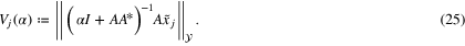
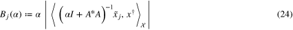
From (16), (23) we can derive the following bound in terms of  :
:

At the same time, it should be noted that  is a monotonically decreasing continuous function of α. Following the analysis given above, we propose a modified version of the balancing principle for the data functional strategy on Tikhonov–Phillips regularization.
Consider the Tikhonov–Phillips regularized data functional  . We choose the value of α from the finite set

according to the balancing principle
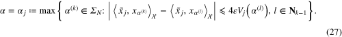
Theorem 3.5. If the value of α is chosen from the finite set  according to the balancing principle (27), then

where the coefficient C can be estimated as
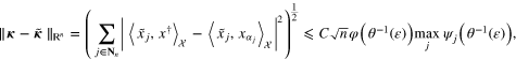
Theorem 3.5 can be proved by the same argument as in [25] (section 1.1.5) and [28]. It leads to the following result.
Theorem 3.6. Suppose that  and φ is such that the function
  is increasing and
  . If
. If  is chosen according to (27) and the bound (16) holds true then
Proof. We shall use (26) to estimate  . We first consider (25). By the assumption of this theorem on the index function φ, using the proof of proposition 2.15 of [25], we observe that for
  , the assumption of theorem 3.4 is satisfied and we have that

where C depends only on the norm of  and
and  is an index function satisfying the assumption of theorem 3.3 in a sense that
  , and the both functions
  and
and  are nondecreasing ones. The existence of such
  is guaranteed by theorem 3.4.
We then estimate (24). Again, from the proof of proposition 2.15 of [25], the following bound

is satisfied, where the coefficient C depends only on the norms  . Theorem 3.5 tells us that if we choose the value of α as per (27) then the error estimate (28) can be achieved. Thus, in view of the bounds (28), (30) and (29) it is clear that
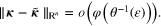
 ![${\theta }^{-1}(\varepsilon )\in [{\varepsilon }^{2},1]$](https://content.cld.iop.org/journals/0266-5611/31/7/075005/revision1/ip514982ieqn234.gif) and
and
proving the desired result. □
It is worth noting that given A and  the value of
  at any point
 ![$\alpha \in (0,1]$](https://content.cld.iop.org/journals/0266-5611/31/7/075005/revision1/ip514982ieqn237.gif) can be calculated directly as the norm of the solution of the equation
can be calculated directly as the norm of the solution of the equation  in the space
  , and it does not require any knowledge of
  .
.
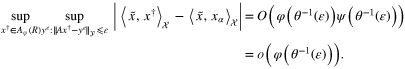
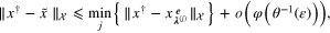
We prove the following main result of aggregation.
Theorem 3.7. Suppose that  is the ideal aggregator in the sense of (9) and xag is its approximant constructed according to (13), (12) and (21). Let ye be an observation that satisfies the bound (16). If
  , where φ is an index function such that the function
  is increasing,
  , and the values of the regularization parameters
  in (21) are chosen according to the balancing principle (27) using only
  and
and  , then
Proof. According to the triangular inequality, we have

We must estimate  . To this end, from (28), (31) we observe that
where C depends only on the norms of  and
and  . Thus, we get
It follows from (11) that

Finally, combining the estimates above, we find that

proving the desired result.
□Theorem 3.7 tells us that the coefficients  of the aggregator xag can be effectively obtained from the input data in such a way that the error
  differs from the ideal error
  by a quantity of higher order than the best guaranteed accuracy of the reconstruction of
  from the most trustable observation (16).
The conclusion of theorem 3.7 also indicates that the error of aggregation  consists of two parts: the optimal approximation error
  and a higher order error
  . On one hand, it is clear that involving more linearly independent solutions in the aggregation helps reducing the optimal approximation error to varying degrees. On the other hand, from the proof of theorem 3.7, it can be seen that the coefficient implicit in the o-symbol increases with n at least as fast as
  . This means that in order to be effective, the aggregator xag should be built on the basis of a modest number of approximations
  . In the context of the Tikhonov–Phillips joint regularization, these approximations correspond to different rules for selecting the values of the regularization parameters
  . The number of such rules is not so large. In our numerical illustrations, we use n = 2. At the same time, we also test the aggregation of the approximations
  corresponding to different values of the regularization parameter in a single parameter regularization scheme. In this case, we use n = 30, and we still observe good aggregation performance.
Note that in our analysis the balancing principle (27) has been used mainly for the theoretical reason. In numerical experiments below the vector  of the coefficients of the aggregator xag is found from the system (12) with (21), where the regularization parameters
  are chosen by a version of the quasi-optimality criterion which is described below: for the functional
  , we choose the value
  from
from

for some  such that

Observe that the balancing principle (27) and the version of the quasi-optimality criterion presented above are similar in the sense that both parameter choice rules operate with the differences of the approximate values  of the quantity of interest
  . A practical advantage of the quasi-optimality criterion is that it does not require the knowledge of the noise level . At the same time, as it was shown in [5], under some assumptions on the noise spectral properties and on
  , the quasi-optimality criterion allows optimal order of error bounds for the Tikhonov–Phillips regularization. On the other hand, theorem 3.3 tells us that, in principle, an error bound of order
  can be achieved with the choice of the regularization parameter α that does not depend on a particular
  . This hints at the possibility to use any of the known parameter choice rules, such as the discrepancy principle, the balancing principle or the quasi-optimality criterion, for achieving a bound of the order
  . In the next section, we demonstrate the performance of the aggregation by the linear functional strategy that is based on the parameter choice rule (32) chosen due to its simplicity.
To close this subsection, we present the method of aggregation, labelled as 'M3', as the third method for the parameter choice. For a series of regularized solutions corresponding to different parameter choices, we do aggregation by using a single observation (16) for the approximation of the objective aggregator with the regularization parameter being chosen by the quasi-optimality method. Algorithm 3.1 is presented below to describe the method.
Algorithm 3.1 for M3
Input:

Output: xag
1: for j = 1 to n do
2: for k = j to n do
3:

4: end for
5: for l = 1 to
 , where
  do
do
6:
 ;
; 
7: if
 then
then
8:

9: end if
10: end for
11:

12: end for
13:
 , where
14: return

3.3. Using aggregation as a feasible solution to the joint inversion problem
With the above discussion, we are now ready to provide a landscape view of the proposed aggregation scheme for the resolvent of the joint inversion problem. Consider the joint inversion problem of multiple observation (1) and (2). We summarize below the general method applied to the joint inversion problem in algorithm 3.2.
Algorithm 3.2 for joint inversion
Input:

Output:

1:
 , for all
2:
 select the most trustable one from input
  , and the corresponding operators
3: return
 call algorithm 3.1 with parameters
Next, we prove convergence of algorithm 3.2.
Theorem 3.8. If n vectors  ,
,  of weighted parameters for the objective functional (5) are provided,
  , where φ is an index function such that the function
  is increasing,
  , and A is the operator corresponding to the most trustable observation chosen from (1), then the aggregation scheme depending only on the given data generates the approximant
  of
of  satisfying
where  ,
,  , are the minimizers of the objective functional Φ defined by (5) with the parameters
  .
.

By using the results of theorem 3.7 with all conditions fulfilled, we have that

and  can be effectively attained by applying the aggregation scheme only depending on the input data: multiple observation (1), (2) and
  . Moreover, by the definition of
  , we obtain that

Combining the above discussion, we get the desired estimate.
□Theorem 3.8 reveals that when coping with a joint inversion problem while several possible weighted parameter vectors for observation errors are provided and the best is not decided, an 'aggregation' approach may achieve a more reliable result. Such an 'aggregation of weighted parameters' is interpreted in a way that it aggregates the solution candidates corresponding to each parameter vector. The 'reliability' is in the sense that the error between the aggregator and the real solution will not exceed the one between the solution candidate corresponding to any single weighted parameter and the real solution, plus a term of higher order than the best guaranteed accuracy of the reconstruction error from the most trustable observation equation one believes. Further, the retrospection of theorem 3.7 also supports that in general, better accuracy of the aggregated solution than any single solution may be expected. The above theoretical suggestions are justified by the numerical tests in the following section.
4. Numerical illustrations
In this section we present numerical experiments to demonstrate the efficiency of the proposed aggregation method and to compare it with other existing methods in the literature. Our numerical experiments are preformed with MATLAB version 8.4.0.150421 (R2014b) on a PC CELSIUS R630 Processor Intel(R) Xeon(TM) CPU 2.80 GHz. All data are simulated in a way that they mimic the inputs of the SST-problem and the SGG-problem described by the equations (1) with (3).
It is well-known (see e.g. [12]) that the integral operators Ai defined by (3) with the kernels  , act between the Hilbert spaces
  and
and  of square-summable functions on the spheres
  , and admit the singular value expansions
where  is the orthonormal system of the spherical harmonics on the unit sphere
  , and
, and

The solution  to (1) with (3) models the gravitational potential measured at the sphere
  , that is expected to belong to the spherical Sobolev space
  (see e.g. [32]), which means that its Fourier coefficients
  should be at least of order
  . Therefore, to produce the data for our numerical experiments we simulate the vectors
of the Fourier coefficients of the solution  in the form
where  are random
  -dimensional vectors, whose components are uniformly distributed on
 ![$[-1,1]$](https://content.cld.iop.org/journals/0266-5611/31/7/075005/revision1/ip514982ieqn322.gif) . In view of (33), the vectors of the Fourier coefficients
. In view of (33), the vectors of the Fourier coefficients
of noisy data  are simulated as
where  are Gaussian white noise vectors which roughly correspond to (2) with
  . All random simulations are performed 500 times such that we have data for 1000 problems of the form (1) with (3). Moreover, we take
  for the radius of the Earth, and
  . All spherical Fourier coefficients are simulated up to the degree k = 300, which is in agreement with the dimension of the existing models, such as Earth gravity model 96 (EGM96). Thus, the set of simulated problems consists of 500 pairs of the SGG- and SST-type problems (1) with (3). In our experiments, each pair is inverted jointly by means of Tikhonov–Phillips regularization (4), (5) performed in a direct weighted sum of the observation spaces
  , and we use three methods for choosing the regularization parameters (weights)
  .
.
In the first method (i.e. M1), we relate them according to (7). Recall that the data are simulated such that  . Therefore, we have
  . Then the parameter
  is chosen according to the standard quasi-optimality criterion from the geometric sequence
  . As a result, for each of 500 pairs of the simulated problems we apply algorithm 2.1 and obtain a regularized approximation to the solution
  that will play the role of the approximant
  .
.
In the second method (i.e. M2), the parameters  are selected from
  according to the multiple version of the quasi-optimality criterion. In this way, for each of 500 pairs of the simulated problems we apply algorithm 2.2 and obtain the second approximant
  .
.
The third method (i.e. M3) consists in aggregating the approximnats  according to the methodology described in the end of section 3.2. In our experiments the role of the most trustable observation equation (15) is played by the equations of the SGG-type (3), (33), i = 2, and we label the aggregation based on them as M3(2). We choose these equations because the data for them are simulated with smaller noise intensity. Then the required regularization parameters
  are selected from the geometric sequence
  in such a way that
  according to the quasi-optimality criterion (32). In this way, for each of 500 pairs of
  we apply algorithm 3.1 and obtain an aggregated solution xag. Note that in general, no specific relation is required between the sets of possible values of the regularization parameters
  and
and  . In this test, we use the same set
  for the sake of simplicity.
We have to admit that the decision, which model to select as the most trustable one, may contribute to the performance of the aggregation method M3. In our discussion, 'the most trustable model' might be (but not limited to) either the least ill-posed observation equation, or the equation with the smallest noise level. If one has a model with both of these features, then one can choose it. However, it may happen that the above features are not attributed to the same observation equation. For example, in our numerical illustrations for (3), (33), (34), the SST-type equation (3), (33), i = 1, is contaminated by more intensive noise, but it is less ill-posed than the SGG-type equation (3), (33), i = 2, which has been chosen by us as the most trustable model. This can be seen from (34) when one compares the rates of the decrease of the singular values  and
and  as
as  ; for the considered values
  (km),
(km),  (km),
(km),  (km) both
  , i = 1, 2, decrease exponentially fast, but
  decreases slower than
  .
.
To illustrate what happens when an alternative model is chosen as the most trustable one, we implement the aggregation method M3 on the base of the SST-type equations (3), (33), i = 1, and label it as M3(1). All other implementation details are exactly as described for M3(2).
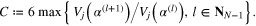
The performance of all four methods is compared in terms of the relative errors  , and
, and  . The results are displayed in figure 1, where the projection of each circle onto the horizontal axis exhibits a value of the corresponding relative error of one of the methods M1, M2, M3(1) and M3(2), in the joint inversion of one of 500 pairs of the simulated problems. From this figure we can conclude that the aggregation by the linear functional strategy can essentially improve the accuracy of the joint inversion compared to the aggregated methods (M3(2) in comparison to M1 and M2). This conclusion is in agreement with our theorem 3.7. At the same time, figure 1 also presents an evidence of the reliability of the proposed approach. Indeed, in the considered case, even with the use of an alternative (i.e. suboptimal) model, the aggregation, this time M3(1), performs at least at the level of the best among the aggregated approximants M1 and M2, as it is suggested by theorem 3.8 and the succeeding comment.
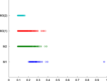
Figure 1. Examples of a joint regularization of two observation models. Relative errors of the regularization by a reduction to a single regularization parameter (M1), the regularization with a multiple quasi-optimality criterium (M2), and the regularization by aggregation (M3(1),M3(2)).
Download figure:
Standard image High-resolution imageIn view that the above rules may only lead to sub-optimal error control, one does not necessarily adhere to these guidelines. Indeed, the terminology 'the most trustable' suggests that one would better consider the selection of an ideal observation in aggregation from multiple perspectives and as an issue of personal preference or need. It actually relies on particular cases.
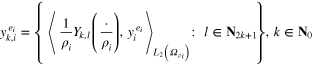
Note that it is also possible to aggregate the approximants  corresponding to different values of the regularization parameter of a one parameter regularization scheme applied to a single observation equation (1). In such a case this equation is also used within the linear functional strategy to approximate the components
  of the vector
  . This method is labeled with M4 and algorithm 4.1 is provided below.
Algorithm 4.1 for M4
Input:
 where
where  is the parameter set
Output: xag
1: for
 to
to  , where
  do
do
2:

3: for
k = 1 to j' do
4:

5: end for
6: end for
7: for j = 1 to
 do
do
8: for l = 1 to
 do
do
9:

10: if
 then
then
11:

12: end if
13: end for
14:

15: end for
16:

17: return
 , where
When applying algorithm 4.1, we use the data simulated as above and for each of 500 equations of the SST-type we construct the candidate approximants  of the form
where  traverses the geometric sequence
  . In one way, we choose the final approximant
  according to the standard quasi-optimality criterion [33], which we label as 'Q1'. Then, in the other way, we continue algorithm 4.1 by performing aggregation upon the candidate approximations
  with the most trustable observation equation being selected by the SST-type problem itself and using the same geometric sequence
  .
.
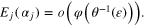
Again the performance of the methods Q1 and M4 is compared in terms of the relative errors  , and
, and  . The results are displayed in figure 2, where the circles have the same meaning as in figure 1. Figure 2 shows that the aggregation based on the linear functional strategy, which is equipped with the quasi-optimality criterion (32), essentially improves the accuracy of the regularization, as compared to the use of the standard quasi-optimality criterion.

Figure 2. Examples of the regularization of a single observation model. Relative errors of the regularization with the quasi-optimality criterion (Q1) and of the regularization by aggregation (M4).
Download figure:
Standard image High-resolution image
It is also instructive to compare figures 1 with 2. This comparison shows that the aggregation of the approximants coming from joint inversion of SGG- and SST-type models outperforms the aggregation of the approximants coming from the single observation model. Clearly, figures 1 and 2 demonstrate the advantage of the joint inversion.
5. Concluding remarks
There is a need to reduce the uncertainty of biases when adopting regularization parameter choice methods, especially in the multi-parameter choice problem arising from the multi-penalty or multi-observation inversion, e.g. joint inversion of multiple observations. It is of no doubt that suitable parameter choices are critical for the accuracy of reconstruction which needs to be considered carefully in practice. Such a matter usually depends on a concrete problem at hand, the a priori information we know from the problem and the method we decide to use. However, unfortunately it is of no hope to gather the whole information usually. Therefore, parameter choice schemes in the light of a priori or a posteriori principles emerge but it seems that not a single one can avoid practice bias and drawback to a certain extent, to the extent of our knowledge. Moreover, different solutions resulted from different parameter choice methods may compensate the flaw of each other. The methodology of aggregation is such a method to meet the above requirements that a more reliable result with more tolerance of the reconstruction error can be expected in a normal circumstance.
We conclude that the proposed linear aggregation of approximate solutions resulting from different methods to the same quantity of interest might allow significant improvement of the reconstruction accuracy and reduction of the uncertainty of possible bias by using a single method. In this connection, it is worth mentioning that concerning the joint inversion of multiple observation models, a standard tool is also the Kaczmarz-type iteration. This tool is based on rewriting the observation equations (1) as a single operator equation and on applying iterative regularization methods that cyclically consider each equation in (1) separately. Note that the Kaczmarz method can be seen as a single-parameter regularization, where the number of cycles is playing the role of the regularization parameter. It has been studied even for nonlinear equations (see e.g. [7, 17]). At the same time, an open question is what happens when the observation equations (1) have different degrees of ill-posedness, as in the case of the SST- and SGG-problems because the resulting rewritten operator equation may inherit the highest ill-posedness among the problems (1). On the other hand, an approximate solution produced by the Kaczmarz iterative regularization can in principle be aggregated with other approximate solutions in the same way as it has been discussed in section 3. In the future, we shall study such aggregation of different regularization techniques.
When viewed from another angle, aggregation might be treated as a third method of the parameter choice scheme among, or an ideal supplement to, the classical and state-of-art parameter choice methods in the literature. But it still needs to point out that the efficiency of aggregation relies on the quality of 'material' to be aggregated and the underlying methods. In this sense, it is reasonable that the extent of 'good quality' and 'bad quality' of the material should be within the tolerance of errors and the extent of linear correlation of the material for aggregation in order to expect a better aggregation which, of cause, might exhibit different effects in practice. Our theory guarantees the aggregation accuracy is not worse than any one by using only a single parameter choice method plus a term of order higher than the best guaranteed reconstruction accuracy from the most trustable observation equation one believes. Our experiments show that the results in practice might be more promising in most general cases.
Acknowledgments
This research was performed when the first author visited Johann Radon Institute for Computational and Applied Mathematics (RICAM) within the framework of cooperation between RICAM and Guangdong Province Key Lab of Computational Science. The stay of the first author at RICAM was supported in part by the Austrian Science Fund (FWF), Grant P25424 and by Guangdong Provincial Government of China through the 'Computational Science Innovative Research Team' program. The research of the third author was supported in part by the United States National Science Foundation under grant DMS-1115523, by the Guangdong Provincial Government of China through the Computational Science Innovative Research Team program and by the Natural Science Foundation of China under grants 11071286, 91130009 and 11471013.