


Abstract
We study the non-equilibrium dynamics of ultracold bosons in an optical lattice with a time-dependent hopping amplitude J(t) = J0 + δJcos(ωt) which takes the system from a superfluid phase near the Mott-superfluid transition (J = J0 + δJ) to a Mott phase (J = J0 − δJ) and back through a quantum critical point (J = Jc), and demonstrate dynamics-induced freezing of the boson wave function at specific values of ω. At these values, the wave function overlap F (defect density P = 1 − F) approaches unity (zero). We provide a qualitative explanation of the freezing phenomenon, show its robustness against quantum fluctuations and the presence of a trap, compute residual energy and superfluid order parameter for such dynamics, and suggest experiments to test our theory.
Export citation and abstract BibTeX RIS
The theoretical study of non-equilibrium dynamics in closed quantum systems has seen great progress in recent years [1] mainly due to the possibility of realization of such dynamics using ultracold atoms in optical lattices [2, 3]. For bosonic atoms, such systems are well described by the Bose-Hubbard model with on-site interaction strength U and nearest-neighbor hopping amplitude J [4, 5]. Several theoretical studies have been carried out on the quench and ramp dynamics of this model [6–11]; some of them have also received support from recent experiments [3]. In contrast, studies on periodically driven closed quantum systems have been undertaken in the past mainly on driven two-level systems [12, 13] or on weakly interacting or integrable many-body systems which can be modeled by them [14, 15]. Among these, ref. [15] has predicted freezing of the time-averaged value of the order parameter (magnetization) of a periodically driven one-dimensional (1D) Ising or XY model, when the temporal average is performed over several drive cycles, at specific drive frequencies. Such a freezing occurs in the high-frequency regime and exhibits non-monotonic dependence on the drive frequency. However, to the best of our knowledge, the phenomenon of dynamics-induced freezing has never been demonstrated for dynamics involving a single drive cycle and/or for non-integrable quantum systems. Recent studies of periodic dynamics of the Bose-Hubbard model have not addressed this issue [16, 17].
In this work, we demonstrate that the periodically driven Bose-Hubbard model may exhibit dynamical freezing of the boson wave function by observing that after one cycle the wave function comes back to its original value ψ(T) = ψ(0) for specific values of the drive frequency ω = 2π/T. Our driving protocol constitutes a time-dependent hopping amplitude of the bosons J(t) = J0 + δJcos(ωt) with J0 and δJ chosen such that the drive takes the system from a superfluid (SF) (J = J0 + δJ) to the Mott insulator (MI) state (J = J0 − δJ) and back through the tip of the Mott lobe where μ = μtip. We provide a semi-analytical understanding of the freezing phenomenon using mean-field theory and compute the defect formation probability P = 1 − F (where F = |〈ψ(t = 0)|ψ(t = T)〉|2 is the wave function overlap), the superfluid order parameter Δ(T) = 〈ψ(T)|b|ψ(T)〉 (where b denotes the boson annihilation operator), and the residual energy Q = E(t = T) − EG (where E(t = T) is the energy of the system at the end of the drive cycle and EG is the initial ground-state energy) as a function of ω. We also show, via inclusion of quantum fluctuation by a projection operator approach [11] and numerical mean-field study of a trapped boson system that the freezing phenomenon is qualitatively robust against quantum fluctuations and the presence of a trap. We also show that such a phenomenon persists for multiple drive cycles. We note that such a freezing behavior has two novel characteristics which distinguishes it from its counterpart in ref. [15]. First it always occurs at low frequencies, i.e., ℏω/U ≪ 1 for all ω for which the freezing occurs. Second, it occurs for a single cycle of the drive. To the best of our knowledge, the dynamics-induced freezing phenomenon at such low drive frequencies and non-integrable models has not been studied in the context of closed quantum systems; our work therefore constitutes a significant advance in our understanding of periodic dynamics of closed non-integrable quantum systems.
The Hamiltonian describing a system of ultracold bosonic atoms confined by a trap and in an optical lattice is given by

where μr denotes the chemical potential at site r, r' denotes one of the z nearest-neighboring sites of r, and  . In the absence of a trap, μr = μ for all sites and for zJ ≪ U, the ground state of the model is a MI state with
  bosons per site with
  for 0 ⩽ μ/U ⩽ 1. For zJ ≫ U, the bosons are delocalized and the system, for d ⩾ 2, is in a SF state. In between, at J = Jc, the system undergoes a SF-MI transition. The equilibrium phase diagram of the model constitutes the well-known Mott lobe structure [4, 5].
To obtain an semi-analytic insight to the freezing phenomenon, we first analyze the periodically driven Bose-Hubbard model in the absence of a trap and within mean-field approximation. The time-dependent mean-field Hamiltonian is given by
where  and Δ'0 = Δ'(t = 0). Within homogeneous mean-field theory, the Gutzwiller wave function for the bosons reads
  [18]. The Schrödinger equation
  yields the time-dependent mean-field equations for fn(t) ≡ fn:

where  , and En = −μn + U(n − 1)n/2. In what follows, we shall choose J0 and δJ such that the ground state of Hmf with J = J0 + δJ is a SF state close to the QCP so that fn(t = 0) ≃ 0 for n ⩾ 3 and f1(t = 0) ≫ f0(t = 0) ,f2(t = 0).
Our strategy for solving these equations will be the following. First, we shall solve the mean-field equations numerically keeping states with n ⩽ 4. Such numerics yields the result that in the MI and SF states close to the QCP all fn(t) for n ⩾ 3 remains small for all t during the dynamics. We shall then use this fact to develop semi-analytic understanding of the freezing phenomenon using equations for f0, f1 and f2 (see footnote 1).
The equations for f0, f1 and f2 then read (suppressing the time dependence of fn(t) for clarity)
Multiplying each of the equations for fn in eqs. (4) by f*n and subtracting the equations thus obtained from their complex conjugates, it is easy to see that |fn|, for n ⩽ 2, obeys the relation

Parameterizing ![$f_n=r_n(t) \exp [i \phi _n (t)]$](https://content.cld.iop.org/journals/0295-5075/100/6/60007/revision1/epl15090ieqn8.gif) , with the choice that ϕn(0) = 0 and rn(0) = fn(0), one can write
, with the choice that ϕn(0) = 0 and rn(0) = fn(0), one can write

where η is a time-independent parameter whose value is fixed by the initial values rn (see footnote 2) Note that η represents the magnitude of the particle-hole asymmetry since r0 = r2 for η = 0. Substituting eq. (6) in eq. (4), we get
where we have suppressed the time dependence of r1 and ϕs(d) for clarity, ϕs = ϕ0 + ϕ2 − 2ϕ1 and ϕd = ϕ2 − ϕ0 are the sum and differences of the relative phases of the Gutzwiller wave function, and the functions gi(r1) are given by
We note that the first two of the equations in eqs. (7) are coupled equations describing the evolution of r1 and ϕs, while the third describes the evolution of ϕd in terms of r1 and ϕs. Furthermore, using a scaled variable t' = ωt/(2π), we find that the relation between r1 and ϕs can be written as

This allows us to symbolically write ϕs = ξ(r1,t'), where ξ is an unknown function, and thus establish an ω-independent relation between r and ϕs for any fixed t'.
Equations (6), (7) and (8) constitute the central result of this work. They constitute a complete description of the evolution of f0, f1, and f2 in the presence of the periodic drive and provide an understanding of the freezing phenomenon as follows. First, we find that a numerical solution of eq. (7), together with eq. (6), allows us to obtain rn, ϕs and ϕd as functions of time. The plots of 1 − r1(t) and ϕs(t) as functions of t for ω/Jc = 0.52 is shown in panel (a) of fig. 1. We find that r1 changes appreciably when J(t) is close to Jc; however, r1(T) ≃ r1(0) at the end of the evolution. Note that this also implies, via eq. (6), that r2(0)(0) ≃ r2(0)(T). Panel (b) of fig. 1 shows that the relation r1(T) ≃ r1(0) holds for a significant range ω/Jc ⩽ 0.8. Second, we note that, ϕs(t) undergoes rapid oscillation when J(t) ⩽ Jc; however, it also comes back close to its initial value at the end of the drive: ϕs(T) ≃ ϕs(0). Since ϕs and r1 satisfies an ω-independent relation, ϕs = ξ(r1,t'), we infer that ϕs must remain close to its initial value for the same range of ω for which r1(T) ≃ r1(0); this is verified numerically in panel (b) of fig. 1. Finally, we note, from the panels (c) and (d) of fig. 1, that ϕd(T) is a monotonic function of ω. Thus, we may define ω = ω*m for which ϕd(T) ≃ 4πm (m being an integer). Together with the fact that r1(T) ≃ r1(0) and ϕs(T) ≃ ϕs(0) = 0, we find that at ω = ω*m, both the relative phases satisfy ϕ2 − ϕ1 = −(ϕ0 − ϕ1) ≃ 2πm leading to |ψmf(T)〉 ≃ |ψmf(0)〉 up to a global phase. This constitutes the dynamics freezing of |ψ〉mf.

Fig. 1: (Color online) (a) Plot of 1 − r1(t) (red dashed line) and ϕs(t) (blue solid line) as a function of t. (b) Variation of 1 − r1(T) (red dashed line) and ϕs(T) (blue solid line) with ω. (c) ((d)) Plot ϕd(t) (ϕd(T)) as a function of t (ω). For all plots J0 = 1.05Jc, δJ = 0.35Jc, and μ = 0.414U.
Download figure:
Standard imageTo obtain an accurate estimate of the degree of freezing and to check the validity of the discussion above, we compute the defect density P = 1 − F = 1 − |〈ψmf(T)|ψmf(0)〉|2 via direct numerical solution of eq. (3) keeping n ⩽ 4 states per site. The plot of P as a function of ω clearly shows that P → 0 at ω = ω*m. A plot of Log10P vs. ω near ω*9/Jc ≃ 0.47, shown in panel (a) of fig. 2, reveals that Log10P ∼ − 6 indicating that the overlap, up to a global phase, is exact within our numerical accuracy. We have checked for all ω*m ⩽ 0.8Jc, Log10P < −4 which indicates a near perfect freezing. We also compute the residual energy Q(T) and the SF order parameter

at t = T as a function of ω. We find from eq. (10) that |Δ| is independent of ϕd. Thus |Δ(T)|/|Δ0| and Q/U (which can also be shown to be independent of ϕd) remain close to unity and zero respectively over the entire range of ω/J for which r1 and ϕs remain close to their initial values as shown in panels (c) and (d) of fig. 2. Such a behavior distinguishes these quantities from P which depends on ϕd and hence vanishes at discrete ωm. Finally, we find that for all values of J0 shown in panel (b) of fig. 2, there is an appreciable range of ω/Jc within which the freezing phenomenon occurs and that ω*m decreases monotonically as a function of J0 over this range.
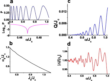
Fig. 2: (Color online) (a) Plot of the defect density P as a function of ω/Jc displaying freezing at ω = ω*m. The inset shows Log10P near ω*9 ≃ 0.47Jc. (b) Variation of ωm/Jc as a function of J0/Jc for m = 6. (c) and (d): plot of Q and |Δ(T)| as functions of ω/Jc. All parameters are the same as in fig. 1.
Download figure:
Standard imageA physical picture of the freezing phenomenon described above can be obtained as follows. The dynamics of the bosons in the MI and the SF phases near the transition constitutes change in both the amplitudes and the relative phases of the different components of the boson wave function. We find that the change in amplitudes after a complete cycle of the drive (at t = T) is close to zero over a range of ω ⩽ Jc. Our treatment of the mean-field equations above brings out the crucial fact that this also means that the change in the sum of the relative phases, ϕs(T), will be small after a complete cycle in this regime since r1 and ϕs are related by eq. (9). In contrast, the difference between the relative phases, ϕd(T), evolves with the drive frequency ω. Thus, at special values of ω = ω*m, where ϕd(T) = 4πm, the mean-field boson wave function comes back to itself after a complete drive cycle leading to freezing.
Next, we study the effect of quantum fluctuations on the freezing phenomenon3. We incorporate such fluctuations by using a projection operator method developed in ref. [11] which provides an accurate treatment of dynamics with fluctuations for zJ(t)/U ≪ 1 (typical value of Jc/U are ∼0.034 for d = 3 and ∼0.061 for d = 2) as seen for linear dynamics in where it provides a qualitative match with experimental results [3]. The idea behind this approach, as detailed in ref. [11], is to introduce a projection operator Pℓ = |n0〉〈n0|r × |n0〉〈n0|r' which lives on the link ℓ between the neighboring sites r and r' of the lattice. Using Pℓ, one can write the boson hopping term as
where P⊥ℓ = (1 − Pℓ). In the strong-coupling regime where zJ(t)/U ≪ 1, the term T'0ℓ[J] = (PℓT'ℓ + T'ℓPℓ), at any instant, represents hopping processes which takes the system out of the instantaneous low-energy manifold. Thus, one can devise a time-dependent canonical transformation via an operator S given by
which eliminates T'0ℓ[J(t)] up to first order in J(t)/U and leads to the effective instantaneous time-dependent Hamiltonian ![$H^{\ast }=\exp (-iS[J(t)]) {\mathcal H} \exp (iS[J(t)])$](https://content.cld.iop.org/journals/0295-5075/100/6/60007/revision1/epl15090ieqn9.gif) . Such a canonical transformation is equivalent to a transformation on the system wave function |ψ〉:
. Such a canonical transformation is equivalent to a transformation on the system wave function |ψ〉: ![$|\psi '\rangle = \exp (-i S[J(t)]) |\psi \rangle $](https://content.cld.iop.org/journals/0295-5075/100/6/60007/revision1/epl15090ieqn10.gif) . We note that |ψ〉 and |ψ'〉 coincides for J = 0 which leads us to the natural choice
. We note that |ψ〉 and |ψ'〉 coincides for J = 0 which leads us to the natural choice  . Note that |ψ〉 is not of Gutzwiller form; it involves spatial correlation due to
 ![$\exp (iS[J(t)])$](https://content.cld.iop.org/journals/0295-5075/100/6/60007/revision1/epl15090ieqn12.gif) factor. The instantaneous energy of the system is given by
factor. The instantaneous energy of the system is given by

and includes O(J2/U2) quantum fluctuation corrections. As shown in ref. [11], this formalism allows one to describe the dynamics of the bosons by solving for the Schrödinger equation for |ψ'〉:

Using the expression of |ψ'〉 and E[{fn}], one can convert eq. (14) to a set of equations for {fnr(t)} [11]. Defining  , one gets
A numerical solution of eq. (15) yields fn(t) and hence |ψ'〉 using which one can compute ![$ |\psi (t)\rangle = \exp [iS] |\psi '(t)\rangle $](https://content.cld.iop.org/journals/0295-5075/100/6/60007/revision1/epl15090ieqn14.gif) perturbatively to O[J(t)2/U2]. Similarly, the expectation value of any operator O at any instant t can be calculated in terms of |ψ'(t)〉:
perturbatively to O[J(t)2/U2]. Similarly, the expectation value of any operator O at any instant t can be calculated in terms of |ψ'(t)〉:

where the ellipsis indicate higher-order terms in J(t)/U. Note that the second term in the expression originates from quantum fluctuation and modifies mean-field result (first term). Using the above-mentioned procedure detailed in ref. [11], we compute P(T), Q(T) and |Δ(T)| as shown in fig. 3. We find that key effects of the quantum fluctuations is to change numerical values of ω*m and the precise range of ω over which freezing occurs; however the mean-field results hold qualitatively in the sense that P → 0 for several ω*m with Log10P ⩽ − 4 for all ω*m. Further ω*m also decreases monotonically with J0 as shown in panel (b) of fig. 3 for ω* ≃ 0.6Jc.

Fig. 3: (Color online) Similar plots as in fig. 2 but with J0[δJ] = 0.87[0.58]Jc and computed using the projection operator approach displaying robustness of the freezing phenomenon against quantum fluctuations. See text for details.
Download figure:
Standard imageNext, we consider the effect of a harmonic trap on the freezing phenomenon. For this part, we numerically solve eq. (3) for d = 2 with μr = μ0 + 0.01U[(rx − 1/2)2 + (ry − 1/2)2], for N0 = 576 sites (linear dimension 24) and with fixed total particle number N0. We choose the trap parameters so that the ground state of the bosons in the center of the trap at t = T/2 is MI phase with  . The evolution of the density profile of the bosons is shown in panel (a) of fig. 4 for t = 0 (left) and t = T/2 (right). Panel (b) of fig. 4 indicates value of ϕd(T) as a function of the position of the bosons in the trap along the line y = 0. The plot shows that for all ω ⩽ 0.3Jc, ϕd evolves coherently with negligible spatial variation. The plots for ϕs and r1 are similar in nature; thus, we expect the boson evolution to have the same qualitative properties as that found within a homogeneous mean-field approach. A plot of P (|Δ(T)|/|Δ0|) as a function of Log10(ω/Jc) in the panels (c), (d) of fig. 4 confirms this expectation. We find that the main effect of the trap is to push the freezing phenomenon to lower frequencies leaving its qualitative nature unchanged. The largest freezing frequency occurs at ≃0.2Jc which is large compared to frequencies ≃0.05Jc where momentum-conserving boson pair production at finite momenta, which is not captured within mean-field theory, is expected to become significant [19]. Figure 4 also demonstrates that the freezing phenomenon disappears at higher drive frequencies where the trapped bosons do not evolve coherently leading to spatial variation of ϕd.

Fig. 4: (Color online) (a) Plot of the boson density profile in the trap at t = 0 and t = T. (b) Variation of relative phase ϕd(T) as a function of the position (along y = 0) in the trap displaying coherent evolution of the bosons. (c) and (d): plots of P and |Δ(T)|/|Δ0| as functions of ω displaying the freezing phenomenon at ω*m. For all plots J0 = 0.04U, δJ = 0.015U, Jc = 0.041U, and μ0 = 0.415U.
Download figure:
Standard imageFinally, we note that the freezing phenomenon persists for multiple periods of the drive. To show this explicitly, we revert to single-site mean-field theory and plot P around a freezing frequency ω* = 0.47Jc for several cycles of the drive in fig. 5. The plot shows that P(ω*) increases with number of drive cycles; however, even after t = 10T, its value remains small (⩽10−4) which indicates that the freezing persists to a good degree of accuracy for longer drive times.

Fig. 5: (Color online) Variation of logP with ω near ω* ≃ 0.47Jc for n = 2 (black solid line), 4 (blue dotted line), 6 (red dashed line), 8 (green dot-dashed line) and 10 (magenta dot-dash-dotted line) periods showing the persistence of freezing for longer drive times. We have found similar behavior when fluctuations are included via the projection operator method.
Download figure:
Standard imageFor experimental verifications of our work, we suggest interference of two bosonic condensates in the presence of an optical lattice, near the QCP which are separated after creation by a double-well potential and allowed to evolve separately for a fixed holdout time. It is well known that recombination of such separated condensates can act as a readout scheme for their relative phases [20]. We propose such a readout when one of the condensates is driven periodically with a frequency ω during the holdout for a single period T = 2π/ω. Our specific prediction is that the relative phase measured for such a drive with ω = ω*m is going to match the phase without any drive indicating dynamics-induced freezing. For all such experiments one needs to estimate an optimal temperature T0 at which they can be carried out. The typical value of U deep inside the Mott phase is ≃2 KHz = 200 nK leading to a melting temperature of Tm ≃ 0.2U = 40 nK for d = 3. The SF phase near the Mott tip has a coherence temperature of Tc ≃ zJc ≃ 35 nK [21]. Thus, a temperature of a few nano-kelvins (T0 ≪ Tm,Tc), which is currently within the experimental reach, would be ideal for testing our prediction.
In conclusion, we have demonstrated that periodic dynamics of the ultracold bosons described by the Bose-Hubbard model leads to dynamics-induced freezing of the boson wave function at specific drive frequencies which are determined by the condition ϕd(T) = 4πm. The freezing phenomenon manifests itself at discrete drive frequencies ω*m ⩽ Jc via the presence of dips in the defect density and can be detected by suitable interference experiments. We have shown that this effect, which can be qualitatively understood using mean-field theory, is robust against quantum fluctuations, as incorporated using a projection operator technique, and the presence of a trap. We note that designing assisted driving protocols for near-adiabatic drives in interacting many-body systems has been the subject of a plethora of theoretical and experimental studies lately [22]. Our work provides a rare example of near-adiabatic driving without assistance4 in an experimentally realizable non-integrable quantum many-body system.
Acknowledgments
SM and KS thanks K. Ray for several stimulating discussions. KS thanks DST for support through grant SR/S2/CMP-001/2009. DP acknowledges support from the Lee A. DuBridge fellowship.
Footnotes
- 1
We note that such a three level approximation is used in a subsequent discussion for obtaining a semi-analytic understanding of the freezing phenomenon; all numerical procedures were carried out keeping five states (n = 0...4) states per site.
- 2
We note that within the single-site homogeneous mean-field theory, the system does not exhibit freezing for η = 0. This behavior originates from the constraint of conservation of the particle number at each site and is not seen in realistic systems with traps where only the total particle number is conserved.
- 3
Note that the effect of quantum fluctuations which we incorporate through the projection operator method is particularly important at the critical point and in the superfluid phase due to the lack of adiabaticity originating from the presence of gapless excitations.
- 4
The phrase "without assistance" means in the absence of the additional Hamiltonian H1 as discussed in ref. [22].