

Abstract
Cross-correlations are thought to emerge through interaction between particles. Here we present a universal dynamical mechanism capable of generating power-law cross-correlations between non-interacting particles exposed to an external potential. This phenomenon can occur as an ensemble property when the external potential induces intermittent dynamics of Pomeau-Manneville type, providing laminar and stochastic phases of motion in a system with a large number of particles. In this case, the ensemble of particle-trajectories forms a random fractal in time. The underlying statistical self-similarity is the origin of the observed power-law cross-correlations. Furthermore, we have strong indications that a sufficient condition for the emergence of these long-range cross-correlations is the divergence of the mean residence time in the laminar phase of the single particle motion (sporadic dynamics). We argue that the proposed mechanism may be relevant for the occurrence of collective behaviour in critical systems.
Export citation and abstract BibTeX RIS

Published by the EPLA under the terms of the Creative Commons Attribution 3.0 License (CC-BY). Further distribution of this work must maintain attribution to the author(s) and the published article's title, journal citation, and DOI.
This article was made open access on 19 February 2014.
Complex systems usually consist of several dynamical components interacting in a non-linear fashion. Cross-correlations are then used in order to explore the inter-dependence in the time evolution of these components measured in terms of specific quantities characterizing each component. In this context, the existence of cross-correlations has been demonstrated in a wide class of dynamical systems ranging from nano-devices [1] to atmospheric geophysics [2], seismology [3], finance [4–8], physiology and genomics [8]. Of special interest is the case of long-range (power-law) cross-correlations (LRCC) which, being scale free, may be associated with the appearance of characteristics of criticality in the dynamics of the considered complex system. Such a behaviour has been observed, among other examples, in price fluctuations of the New York Stock Exchange during crisis [8], physiological timeseries of the Physiology Sleep Heart Health Study (SHHS) database [8], the spatial sequence describing binding probability of DNA-binding proteins to genes at different locations on mouse chromosome 2 [8] and in flocks of birds [9]. All these findings indicate that the presence of power-law cross-correlations is a quite general property of the dynamics of complex systems. Even more, very recently geometry-induced power-law cross-correlations have been also observed in a coarse-grained description of the dynamics of an ensemble of non-interacting particles propagating in a Lorentz channel [10]. This clearly poses the question of the origin and mechanisms of cross-correlations in particle systems.
Up to now the theoretical treatment of cross-correlations is based on statistical approaches and their microscopic origin is to a large extent unclear. In the following, we identify the dynamical mechanisms leading to LRCC and show specifically that intermittent dynamics, characterized by long intervals of regular evolution (laminar phases) interrupted by short bursts of abrupt evolution (irregular phases), obeyed by each component separately, generates LRCC between the different components, even if they do not interact with each other. It is argued that the emergence of LRCC is of geometrical origin: in a system with a large number of particles the ensemble of their intermittent trajectories forms a random fractal set in time. The two-point correlation function of this set can be identified with the cross-correlation function between intermittent trajectories of different particles which appear in the set with probability one. In addition we provide strong evidence that a sufficient condition for the emergence of such scale-free LRCC is the divergence of the mean length of the laminar phase in the intermittent dynamics of each component.
The prototype model we will use to demonstrate our arguments is a system of N non-interacting particles each with an one-dimensional phase space determined by the variable  . We do not further specify
  : in a real system it can be for example the position or the momentum of particle i or any other property characterizing its state (partially or totally). For the time evolution of
  of each particle independently we use a version of the well-known Pomeau-Manneville map of the interval [11], which has been employed in the literature for the description of a wide class of phenomena ranging from anomalous diffusion to turbulence and spiking behaviour of neuro-biological networks, given as
for  . In eq. (1)
  are positive constants,
  are characteristic exponents fulfilling
  and
and  are random numbers uniformly distributed in (0, 1]. The quantity
  represents the upper border of the phase space region
  within which the evolution of the particle dynamics is laminar. A typical characteristic of the intermittent dynamics is that for any trajectory and for
  the x-values in the laminar region are very close to the diagonal
  since the increase
  of
of  there is very slow. Notice that in eq. (1) there is no coupling term between phase space variables of different particles since there is no mutual interaction. This simple model, based on the normal form for the description of intermittent dynamics, is very general and captures all the basic dynamical ingredients necessary for the development of cross-correlations as we will see in the following. To avoid unnecessary complexity we further simplify the model assuming:
  and
and  for all i. Note that the end of the laminar region
  is not strictly defined. One possible choice, which we use in the following, is to fix
  as the pre-image of 1, i.e. as the solution of the equation
  . A second choice is to set it equal to
  being the x-value for which the non-linear term in eq. (1) becomes equal in magnitude with the linear term. These two values (
 and
and  ) are close to each other (with an at most 20% relative deviation) for almost all values of z and our results for the cross-correlations, shown below, do not depend on this choice.
Using eq. (1) we evolve the considered particle system in discrete time. Different particles correspond to different trajectories, i.e. trajectories starting from a different initial condition. Thus we propagate a set of N trajectories forming the corresponding ensemble. We use the notation  in order to indicate with the index A the possibility for using different representations for an ensemble trajectory for the calculation of the cross-correlation function(s). For example we will use either the original trajectories generated by eq. (1) taking real values in (0, 1) (in this case we use the symbol x for the index A) or a binary representation of these trajectories taking the values 0 in the laminar phase and 1 in the irregular phase (in this case we use the symbol s for the index A). The cross-correlation function is then defined as
where 〈...〉 denotes time averaging while  and
and  are the standard deviations of the trajectories
  and
and  , respectively.
We calculate the cross-correlation function  for various values of z using ensembles of 104 trajectories with length 105 for each case ensuring convergence of our results. For z > 2 we find an algebraic decay of
  with increasing m, having an exponent which depends on z. This conclusion is established by fitting the numerical results with a power-law model and then performing a Kolmogorov-Smirnov test for the normality of the residuals. The obtained p-values are all higher than 0.5, indicating that the power-law is indeed a good fit. The behaviour of
  for z < 2 is more complicated. For
  long-range cross-correlations exist, however they do not possess a power-law form. For
  the cross-correlation function practically vanishes, performing small amplitude random oscillations around zero. It is worth to mention here that a distinction between the properties of intermittent dynamics for
  ,
,  and
and  has been already discussed in [12] where the term sporadicity is introduced for the description of the z > 2 case.
In order to analyze and understand the different behaviour of the cross-correlation functions for z > 2 and z < 2, we consider the distribution of the laminar phase lengths, or as it is often also named, the distribution of the waiting times in the laminar region. It is well known that this distribution obeys asymptotically  a power-law of the form
  [13,14], where ℓ is the laminar phase length. For z > 2 the mean laminar length
  diverges, while for z < 2 it is finite1
. Thus, the divergence of
diverges, while for z < 2 it is finite1
. Thus, the divergence of  should be related with the emergence of power-law cross-correlations between the particles. As we will see later utilizing a simple stochastic description allowing also for analytical treatment, this property can be formulated as follows: if
  is infinite, then the conditional probability that the particle j at an instance n + m is in the laminar region, provided that the particle i was in the laminar region at instance n, is finite and decays algebraically with increasing m.
To facilitate analysis it is useful to develop a symbolic code for the intermittent dynamics in eq. (1). Such a symbolic representation of the dynamics of the Pomeau-Manneville intermittent map capturing several details like the re-injection rate in the laminar region (and therefore the invariant density in the immediate neighbourhood of the marginally unstable fixed point) has been proposed in [12]. Here we are interested mainly to isolate the dynamical properties leading to the emergence of cross-correlations avoiding the influence of other detailed aspects of the intermittent dynamics. Therefore, we will use a much simpler code, mapping x in the laminar region ![$(x \in [0,x^*])$](https://content.cld.iop.org/journals/0295-5075/105/2/26004/revision1/epl16043ieqn43.gif) to 0 and x out of the laminar region
to 0 and x out of the laminar region ![$(x \in (x^*,1])$](https://content.cld.iop.org/journals/0295-5075/105/2/26004/revision1/epl16043ieqn44.gif) to 1. Such a code has been used in [14] to calculate power-spectra of intermittent systems. In practice we use the full dynamics of eq. (1) to generate the ensemble of intermittent trajectories and then we replace the x-values in each time-series by 0 or 1 according to the previously described rule. Subsequently, we calculate the cross-correlation function
to 1. Such a code has been used in [14] to calculate power-spectra of intermittent systems. In practice we use the full dynamics of eq. (1) to generate the ensemble of intermittent trajectories and then we replace the x-values in each time-series by 0 or 1 according to the previously described rule. Subsequently, we calculate the cross-correlation function  for different z-values using the binary sequences generated by the symbolic dynamics from the trajectories of the map in eq. (1).
Complementary we introduce a simple stochastic model containing only the information of the laminar length distribution to simulate the emergence of cross-correlations. We assume a process consisting of two phases defined as follows: i) a stochastic variable ξ takes the value 1 in the irregular phase and the value 0 in the laminar phase and ii) the length of the irregular phase is always 1, while the laminar length probability density is a power-law with exponent  , z being the exponent in the intermittent map of eq. (1). Then we generate an ensemble of realizations of this process and calculate the cross-correlation function
  for this ensemble. Here the index r indicates that the ensemble of trajectories used to calculate this cross-correlation function is generated by the underlying random process. Despite the simple form of both, the intermittent dynamics in binary representation and the associated stochastic process, large scale computational efforts (105 trajectories have been propagated for 106 iterations) are needed to achieve convergence of the long-time behaviour of the cross-correlation function. In fig. 1 we show the results obtained for
  with
with  for
for  . The coloured triangles correspond to A = s, while the red lines to A = r. We observe a very good agreement between the two results for each z value, providing a strong indication that the key quantity determining the scale properties of the cross-correlation function is indeed the laminar length distribution, which is the only quantity shared by the two descriptions.
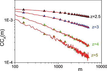
Fig. 1: (Colour on-line) The cross-correlation function  for the symbolic dynamics generated from the intermittent map of eq. (1) (A = s, triangles) and for the stochastic process defined in the text (A = r, red lines) for four different values of z:
  (black), z = 3 (blue), z = 4 (olive green), z = 5 (dark yellow). For the numerical simulations we used an ensemble of 105 trajectories each of length 106.
Download figure:
Standard imageA geometrical interpretation of the emergence of power-law cross-correlations can be obtained by showing that the ensemble of trajectories generated either by the intermittent model of eq. (1) or by the simplified stochastic model introduced above, are realizations of a random fractal set. Thus they can be produced by an automaton [15] and they can also be mapped to a scale-free network using the visibility [16], or the recently generalized cross-visibility algorithm [17]. Adopting this point of view, it is natural to expect that two intermittent trajectories (corresponding to two different particles) being two different subsets of a random fractal set or of a scale-free network are power-law cross-correlated. In fact these long-range cross-correlations are dictated by the power-law form of the two-point correlation function of the corresponding set (random fractal or scale-free network).
To demonstrate the fractal properties of the ensemble of trajectories of the simplified stochastic model, we employ techniques used for the calculation of the lower entropy dimension (LED) [18] for random fractal sets. LED corresponds to the "mass dimension" of usual fractal sets (like for example the Cantor set). Thus, a time-series of length L represented by a sequence of binary symbols (0 for laminar phase and 1 for irregular phase in our case) is interpreted as a set of unoccupied (0) and occupied (1) non-overlapping cells of the embedding set2
. In a large ensemble of trajectories all of length L and generated using a fixed value of z, one can calculate the mean number of "1"s  (averaging over the ensemble) determining the mean number of occupied cells necessary to cover entirely the so defined random fractal set. Notice that the concept of the "random fractal set" establishes only at the level of the ensemble and it is not defined for individual trajectories.
  scales with the length L of the embedding set as

where s is a positive constant and dF is the associated fractal LED. To verify that the ensemble of intermittent trajectories defines a random fractal set, we calculate the mean number of "1"s  for 106 trajectories generated with a fixed z-value and possessing a fixed length L. Then we vary the length of the ensemble trajectories from 102 to 106 calculating for each case
  . We use the same statistics (106 trajectories) to construct the trajectory ensemble for each L-value. In fig. 2(a) we show the result for z = 3 on double logarithmic scale.
We observe a linear behaviour corresponding to a perfect power-law with  . This suggests the validity of a general scaling relation of the form

were the fractal LED may depend on z and the index RF indicates the associated random fractal set. We have performed the fractal LED calculation for several values of z in the range  . Our results are summarized in fig. 2(b), where we show the dependence of the fractal LED
  on the exponent of the intermittent dynamics z. Notice that the power-laws
  for different z's are all of the same quality as measured by the coefficient of determination and the corresponding chi-square per degree of freedom
  of the fit.

Fig. 2: (a)  vs. L for an ensemble of 106 trajectories generated using z = 3 and (b) the fractal LED
  vs. z.
Download figure:
Standard imageThus, we conclude that the ensemble of the intermittent trajectories is equivalent with respect to its complexity with a random fractal set with variable dimension  depending on the characteristic intermittency exponent z. Clearly, the observed fractality refers to the time-dependence, i.e. the considered sets (ensembles of trajectories) are fractal in time. This geometrical property makes transparent the existence of cross-correlations among the members of the ensemble. The fractal LED becomes equal to the embedding dimension for
  signalling the absence of long-range cross-correlations in this case. As already mentioned, in the region
  long-range cross-correlations still exist, however there is no clear signal of a power-law form3
. This issue requires more extensive studies and it is left for a future detailed study.
long-range cross-correlations still exist, however there is no clear signal of a power-law form3
. This issue requires more extensive studies and it is left for a future detailed study.
Going one step further in our analysis, one can develop a method to find an analytical estimation of the cross-correlation function  based on the above introduced stochastic model. To achieve this, let us first consider two binary sequences
  and
and  generated by the stochastic model. To simplify the notation we will omit the index r of the trajectory values for the following steps. The function
  should be proportional to the joint probability
  that the random variable
  has the value 1 at time step k and the random variable
  has the value 1 at time step k + m, averaged over the time
Obviously it holds

since  and
and  are statistically independent. To calculate
  one can use the method introduced in [14] writing

where  is the conditional probability to have a laminar phase of length n directly after the instant k − n if
  has the value 1 at the time instant k − n. The appearance of a laminar phase with duration n is independent of the value of
  at the instant k − n. Thus, we find

where  is the laminar length distribution normalized to one. Inserting eq. (6) into eq. (5) we obtain
which can be solved recursively using as initial condition  with
with  . A similar equation is obtained also for
  replacing simply k with k + m. Having solved eq. (9) one can calculate the left-hand site of eqs. (6), (7) and insert the obtained results in eq. (5) to get an analytical approximation for
  containing three sums. The validity of the introduced analytical scheme is tested in fig. 3, where we show the symbolic dynamics result
  together with the analytical estimation for
  using z = 3.
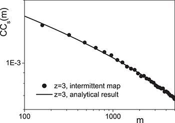
Fig. 3: The cross-correlation functions  (symbolic dynamics, intermittent map, black circles) and the analytical estimation of
  (solid line) for z = 3.
Download figure:
Standard imageWe observe a very good agreement between the analytical result and the numerical simulations for  . Notice that numerically calculated
  is not shown in this plot. However, as illustrated in fig. 1 the numerical results for
  and
and  are very close to each other for any considered z and therefore, the analytical estimation of
  can be also used as an analytical estimation of the cross-correlation
  . The analytical treatment leads us to the conclusion that it is the long-range character of the correlation between
  and
and  existing for any pair of intermittent trajectories which generates the observed cross-correlations. Note that this property has been discussed in [19] in a different context.
With our analysis we have demonstrated a mechanism to establish power-law cross-correlations between particles which do not interact with each other. This phenomenon is induced by the strong intermittent dynamics performed by each of the particles independently. The resulting ensemble of trajectories for all particles, despite the absence of a coupling between trajectories of different particles, forms —in a binary representation— a fractal set in time and the underlying self-similarity leads to the establishment of algebraically decaying cross-correlations. Strong intermittency (sporadicity) discussed here is a result of the interaction of a particle with a suitable external potential (field)4
. The appearance of long-range cross-correlations deems sporadic dynamics a plausible mechanism for the collective behaviour emerging in a N-particle system. Furthermore, since such a collective behaviour is accompanied by scale-free inter-particle correlations, it could be related to the emergence of critical behaviour in the considered system. In fact, a connection of intermittent dynamics with criticality has already been established in [20] using the example of the 3D Ising model. There it has been shown that the order parameter fluctuations at the critical point can be efficiently described by an intermittent map of Pomeau-Manneville type —similar to that of eq. (1)— with additive noise. The exponent z in this intermittent map is related to the isothermal critical exponent δ associated with the second-order transition. This property sets a bound  necessary for the occurrence of critical behaviour. It is remarkable that this bound coincides with the bound obtained by our present analysis in order to have a divergent mean laminar length. An astonishing feature of our results is that the power-law cross-correlations emerge even without interaction among the particles. In the context of critical phenomena such a property is welcome, since it could explain universality aspects. Indeed the microscopic interactions between the elementary degrees of freedom of a critical system do not play any role for the determination of the critical exponents and the associated scaling laws describing the phenomenology of an extended system at the critical point.
In the framework of our approach the obtained correlations are determined by the time evolution of the trajectories of two different particles. To enable a closer relation to equilibrium critical phenomena one should extend these ideas also to the case of a field depending both on time and on space. Such an extension requires the use of matrix equations for the field evolution replacing the variable  by a scalar field
  , where i is a spatial variable, while n is the time variable. At a first glance one could argue that for the calculation of the spatial cross-correlations one might exchange the role of spatial and temporal variables in the dynamics, use eq. (1) to describe changes of the field ϕ in space and average over the time variable. This would lead to power-law cross-correlations between the field values at different locations, which is typical for a critical system. However, a consistent treatment of this case requires more elaborate and extensive studies left for future investigations.
Acknowledgments
This work was made possible by the facilities of the Shared Hierarchical Academic Research Computing Network (SHARCNET: www.sharcnet.ca) and Compute/Calcul Canada. The authors thank C. Petri and B. Liebchen for fruitful discussions. The performed research has been co-financed by the European Union (European Social Fund —ESF) and Greek national funds through the Operational Program "Education and Lifelong Learning" of the National Strategic Reference Framework (NSRF) - Research Funding Program: Heracleitus II. Investing in knowledge society through the European Social Fund. The authors also thank the IKY and DAAD for financial support in the framework of an exchange program between Greece and Germany (IKYDA 2010) and the UK EPSRC for funding under grant EP/E501311/1.
Footnotes
- 1
We refer here to the divergence implied by the asymptotic behaviour for
 . In the small ℓ region there is always a natural cut-off since .
 - 2
The embedding set is the set of L cells.
- 3
This may be attributed to the fact that the corresponding fractal LED approaches the embedding one.
- 4
This could be also a mean field generated by particle-particle interactions.

