


Abstract
We present a path-integral approach for finding solutions of the convection-diffusion equation with inhomogeneous fluid flow, which are notoriously difficult to solve. We derive a general approximate analytical solution of the convection-diffusion equation which is in principle applicable to arbitrary flow profiles. As examples, we apply this approximation to the diffusion in a linear shear flow and in a parabolic flow in infinite space, and to the diffusion in a linear shear flow over an impenetrable interface. This last case is particularly important for problems involving diffusive transport towards an interface with advection. We compare the analytical approximation with numerical solutions which are obtained from a conventional finite-element time-difference method.
Export citation and abstract BibTeX RIS
Introduction
Convection-diffusion equations occur in many physical and chemical problems and describe the transport of heat, matter, or other physical quantities due to a convective flow superimposed by the diffusion of the transported entity within the flow [1]. Only in exceptional cases is the convection-diffusion equation solvable by analytical means [2], but in most cases one has to take recourse to rather complicated numerical integration schemes. These numerical approaches include a wide array of sophisticated finite-element methods [3–12], lattice Boltzmann methods [13], particle methods [14], or solving the related Smoluchowski-Langevin stochastic differential equation [15], see also the overviews [16,17] and the excellent review [18]. In the present paper, we develop a path-integral–based approach to handling convection-diffusion equations and find a general approximate solution of the equation. We demonstrate our method on several examples, and consider in particular the diffusion within an advective shear flow profile over an interface. This problem is particularly important when dealing with the diffusion of molecules or particles close to the surface of microfluidic and nanofludic devices [19,20], or wetting and spreading phenomena [21].
The paper is organized as follows: In the next section, we present our general path-integral treatment of the diffusion-convection equation in two dimensions with an inhomogeneous flow along one direction (uni-directional flow). We obtain a general solution of the problem via a Fourier amplitude function that is expressed as a path integral involving the flow function. By using a second-order cumulant expansion, this path integral can be solved and yields a closed-form analytical approximation of the solution. Next, we apply our approximation to several examples and compare it with exact finite-element numerical solutions. Finally, we discuss our results and possible generalizations and extensions to more complex convection-diffusion problems.
Path-integral formulation
In particular, we consider the convection-diffusion equation

where  is the local concentration of the transported and diffusing quantity at position r and time t, D is the diffusion coefficient, and v(z) is the z-dependent flow profile of a flow along the x-direction. For simplicity reasons, we restrict ourselves here to considering only two spatial dimensions, x and z, but the generalization to the third dimension will be straightforward. Also, we assume that the flow is directed only along the x-direction, but with an arbitrary flow profile v(z) as a function of the coordinate z. Green's function for this equation with the initial condition
  can be written in path-integral form as [22]
where the functional S is defined by

where the path integration in eq. (2) runs over all possible trajectories starting at position  at time zero and ending at position
  at time t. When considering a subset of all trajectories
  with one and the same
  , the path integration over
  can be done analytically yielding the result
where the quantity  is the flow transport along the x-direction measured along the specific trajectory
  which is equal to
Thus, the final solution  is found to be
where the weight function  is given by the path integral
Thus, in each plane  , the solution
  is a superposition of Gaussian distributions with the distribution function
  at center positions
  along the x-axis. Now what remains is to find an analytical solution for the weight function
  . As we will see below, this can be done exactly for specific flow profiles v(z), but also in the general case of an arbitrary flow profile, the path integral of eq. (6) can be analytically approximated, which will be the topic of the next section.
Gaussian approximation
To find an analytical approximation of eq. (6), we switch first to Fourier space by

Now, the Fourier amplitude  is given by the path integral
To approximate this expression analytically, let us formally define the average over a functional ![$V[z(t')]$](https://content.cld.iop.org/journals/0295-5075/108/4/40007/revision1/epl16703ieqn21.gif) by
by
The path integral in the denominator can be calculated analytically and is equal to
Thus, the Fourier transform  can be represented as an average over a functional in the form
The important next step is to apply a cumulant expansion to eq. (11) and to retain only the linear and the quadratic terms of the expansion:
where the linear term is explicitly given by
and the quadratic term by

where the second moment is
With this cumulant approximation, eq. (12), one can back-transform  into real space yielding an analytic expression for the weight function w:
Then, the final approximation for Green's function of the convection-diffusion equation is found to be
where  and
and  are themselves functions of zi, zf, and t as given by eqs. (13)–(15). Equation (17) is the core result of the present paper and approximates the solution of the convection-diffusion equation by a superposition of Gaussian distributions shifted along x by the mean value
  which itself depends on the initial position zi, and on the final position zf where the solution is evaluated. Also, in addition to the spreading of the profile due to pure diffusion, 2Dt, there occurs a convection-induced spreading
  which also depends on zi and zf.
Examples
Let us first consider the special case of a linear flow profile  in free space. In that case, an exact solution is well known [23], and we will reproduce it here on the basis of eq. (17). For the linear profile, both the average
  and variance
  can be calculated exactly:


Moreover, for the linear profile, all higher cumulants are zero. Thus, in that case, the approximate solution given by eq. (17) is the exact solution. The left column of images in fig. 1 shows the temporal evolution of an initially Gaussian concentration profile with unity variance and center position  for the time values
  and 8.

Fig. 1: (Colour on-line) Temporal evolution of the Gaussian concentration profile in three different flow profiles: linear shear flow  (left column), parabolic flow profile
  (middle column), and linear kink profile
  (right column). The value of diffusion coefficient was set to one.
Download figure:
Standard imageNext, let us consider the parabolic flow profile  in free space. Again, both the average and variance can be calculated analytically yielding


However, now the higher-order cumulants do not vanish anymore, and eq. (17) is indeed only an approximation to the exact solution. The temporal evolution of this approximation is shown by the images in the middle column of fig. 1. To compare it with the exact solution, we integrated the full two-dimensional convection-diffusion problem with a finite-element numerical equation solver (COMSOL) on a grid stretching from  till x = 80 and
  till z = 20 with a grid spacing of
  and a time-step of 0.01. The full calculation between t = 0 and t = 8 lasted for 90 min on an Intel(R) Xeon(R) E5440 2,83 GHz quad core PC. For better visualization, we do not compare the full concentration distribution of the numerical calculation and the approximation, but the concentration profiles integrated along the z-axis. The result is shown in fig. 2. It should be noted that the concentration profiles integrated along the x-axis are identical because the integral of eq. (17) along x yields the exact result, independent of the particular function v(z). As can be seen, the approximation eq. (17) matches fairly well the dispersion of the concentration profile for small time values, and starts to deviate sensibly from the exact values only for large time values
  .
.
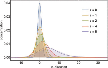
Fig. 2: (Colour on-line) Comparison between the result of a full numerical integration of the convection-diffusion equation with a parabolic velocity profile  and the approximate solution, eq. (17). Shown are the concentrations profiles integrated along the z-direction as a function of the x-coordinate for five time values
  . Solid lines are the exact, numerically integrated solutions, and shaded curves are the result of the Gaussian approximation.
Download figure:
Standard imageAs a last example, we consider a linear flow profile over a planar surface with no-slip condition (flow velocity is zero on surface). This is the most relevant case for all convection-diffusion problems close to an interface. Instead of considering the convection-diffusion equation in a half-space z > 0 with flow profile  , we will treat it in infinite space but assuming the cusp-like flow profile
  . When additionally imposing a mirror-symmetric initial distribution
  , the solution to this problem will be equivalent to the solution of the equation in half space over an impenetrable boundary. Now, there is no more an explicit analytical solution for the average
  and variance
  . Both quantities have to be computed numerically using eqs. (13)–(15). From eq. (13), we find the integral
where we have introduced the abbreviation
This integral has to be evaluated numerically. Because the final result depends on three variables, namely zf, zi and time t, this could be a formidable task. However, the problem is much simplified when realizing that  has the following time-scaling property:

Thus, one has to evaluate eq. (22) only for one specific value of time, t = 1, and can then find the function for all other values of time using eq. (24). Knowing  , one uses next the last equality in eq. (15) for numerically calculating the second moment
  and thus the variance
  . And similar to the average value
  , one can use the time-scaling behavior of the variance,

for finding the function for arbitrary time values. The right column of images in fig. 1 shows the result for the temporal evolution of the Gaussian initial concentration profile for a linear cusp flow with  . The whole calculation took ca. 100 s on the computer. For comparison, we solved the full problem, as before, using the finite-element numerical equation solver COMSOL, where the full calculation again took ca. 90 min. Figure 3 shows a comparison of the temporal evolution of the z-integrated concentration profiles as obtained by full numerical integration and using the approximation (17). Again, the approximation yields fairly good results for small time values and starts to deviate visibly from the exact solution only for
  .
.
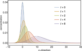
Fig. 3: (Colour on-line) Same as fig. 2 but for a linear cusp velocity profile  .
.
Download figure:
Standard imageDiscussion and conclusion
The core result of our paper is the approximate solution of the convection-diffusion equation (1) as given by eq. (17). The found approximation is very similar to the famous Taylor-Aris approximation for the convection-diffusion induced broadening of plug flow in capillaries [24,25]. There, the concentration profile along the flow direction is also approximated by a Gaussian distribution, for which the peak position and width are derived as functions of time. Furthermore, the physical meaning of the Gaussian approximation found in the present work is also similar to Taylor-Aris dispersion: The Gaussian approximation works very well as long as the diffusion transversal to the flow direction is fast enough for mixing the diffusing molecules perpendicular to that direction before the flow gradient disrupts the profile. To quantify this, one introduces the Péclet number,  , where
  is the mean flow velocity, L the transversal size of the capillary, and D the diffusion coefficient, which describes the ratio of diffusive to convective transport. As long as the Péclet number is small, i.e. as long as the diffusive transport perpendicular to the flow direction dominates over the convective transport, the Taylor-Aris approximation works well. In our examples considered in the present letter, there is no intrinsic lateral size L, because the considered systems are unbounded. However, we consider the transport of an initial Gaussian distribution with distribution width
  . The width of this distribution perpendicular to the flow direction evolves as
  , and we can take
  as the momentous characteristic transversal size of the problem. Then, the average flow velocity over this length scale is proportional to
  for the linear cusp velocity profile, and to
  for the parabolic velocity profile. Thus, one can define the time-dependent Péclet number
  and
and  for the linear and for the parabolic flow profile problems, respectively. As long as these numbers are less or on the order of unity, the Gaussian approximation will work well. But this simple analysis also shows that the fidelity of the approximation deteriorates with time approximately proportional to t for the case of the linear cusp profile, and proportional to
  for the case of the parabolic profile. The main reason is that we considered here only unbounded problems. For a bounded system, where diffusion will be limited in space perpendicular to the flow direction, the approximation will work over longer time-scales, similar to the Taylor-Aris case with low Péclet numbers.
This leads to another important discussion: The approach presented in this letter can be easily generalized to any problem where the convection-diffusion problem can be formulated as

where  form an orthogonal coordinate system and
  being the part of the Laplace operator not containing any derivative with respect to x. Then the function g in eqs. (13), (15) is the fundamental solution of the transverse diffusion problem

and the integration in these equations extends over all transverse coordinates  . Importantly, this concept is also applicable to transversally bounded problems such as shear flow between two parallel plates moving laterally with respect to each other.
Finally, we want to emphasize that the new path integral representation of the solution as given by eqs. (5), (7) and (8) can be used also for finding other exact solutions of convection-diffusion problems, in particular for all cases where the path integral (8) can be evaluated analytically, or for devising efficient numerical integration schemes.
Acknowledgments
Financial support by the Deutsche Forschungsgemeinschaft is gratefully acknowledged (SFB 937, project A5). NK thanks the Niedersächsische Ministerium für Wissenschaft und Kultur for an MWK stipend.