


Abstract
In the present study, we investigate patterns in the postural sway that characterize the static balance in human beings. To measure the postural sway, sixteen healthy young subjects performed quiet stance tasks providing the center-of-pressure (COP) trajectories. From these trajectories, we obtained the COP velocities. We verified that the velocity distributions exhibit non-normal behavior and can be approximated by generalized Gaussians with fat tails. We also discuss possible implications of modeling COP velocity by using generalized Fokker-Planck equations related to Tsallis statistics and Richardson anomalous diffusion.
Export citation and abstract BibTeX RIS
In daily life, we perform several tasks that demand a constant maintenance and control of postural balance (e.g., walking, dancing, carrying shopping bags, and so on). From a biological point of view, the quiet upright stance requires of the body the control of the musculoskeletal system. Such control is possible when the central nervous system processes visual, vestibular and somatosensory information, and uses it to select and control the appropriate postural response [1–5].
The study of postural sway by using center-of-pressure (COP)-based measures has been useful to characterize the dynamics of the postural control system associated with maintaining balance during quiet standing. The dynamics of COP position, which is frequently related to a random walk, has been investigated using a variety of techniques [6–16]. In particular, some studies have focused COP velocities instead of trajectories. It has been argued that COP velocity is most accurate than position or acceleration to modulate human quiet stance [17–19]. Several characteristics of COP velocity, including temporal correlations, have been explored [19–25]. However, investigations related to velocity distributions are scarce. For instance, there are statistical significance tests indicating that COP velocity distributions are non-Gaussian [26,27], but more details about the shape of these distributions have not been studied. The present study is mainly directed to investigate COP velocity distributions.
In this work, sixteen healthy subjects participated in the experiment (eight females and eight males between twenty and twenty-eight years old). After the ethics committee of the Universidade Estadual de Maringá approved the study, all participants gave their informed consent prior to their participation. All participants received oral and written instructions about the experimental protocol. They signed a commitment consenting before performing the tasks of the experiment.
The volunteers stood barefoot and were asked to maintain quiet upright posture on the force platform at a distance of about 1.5 meters from a fixed point in the horizontal plane with their legs oriented in parallel at hip width apart. Each subject was submitted to this task for 60 s, and the same was repeated 10 times in an alternating fashion, i.e., participants took turns among themselves in order to alleviate signs of fatigue. Thus, a total of N = 160 time series for this experiment was obtained. Data were collected using a force platform (EMG SYSTEM do Brasil) to record the ground reaction forces with an acquisition rate of 100 Hz.
The collected COP trajectory time series were filtered by a low-pass filter with a cut-off frequency of 20 Hz. This procedure eliminates high-frequency fluctuations. We then considered a sampling frequency of 50 Hz. The velocity series were obtained by differentiating the position series. The velocity time series were visually examined and it was decided that the first 1.5 second of each series would be removed to avoid anomalies related to the destabilization of the subject at the beginning of the experiment.
A representative COP trajectory is displayed in fig. 1(A) for a subject. Although COP presents a two-dimensional behavior, we chose to emphasize the investigation on its velocity in the anteroposterior direction (forward and backward body movement) as each individual has a higher propensity to imbalance. By using Yt and  to represent two consecutive terms of the COP position series in the anteroposterior direction, one has
  as an element of the series of successive increments. The increment
  will be referred to as COP velocity (
 is proportional to the velocity). Figure 1(B) shows a typical position series and its corresponding velocity series for the anteroposterior direction. Moreover, standardized increments (standardized velocity) are written as
  , where μ is the mean value and σ is the standard deviation of
  . Points above six standard deviations were ignored in all series because it was understood that these data include involuntary stimulation of the subjects.
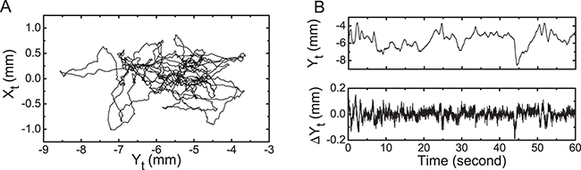
Fig. 1: (A) A typical 60 s center-of-pressure (COP) trajectory, where Xt and Yt correspond to the mediolateral and anteroposterior directions, respectively. (B) The time series of the COP position filtered by a low-pass filter (top), Yt, and its corresponding velocity series (bottom),  .
.
Download figure:
Standard imageThe asymmetrical character and "peakedness" for each COP velocity series were studied. It was also adopted another way to quantify the probability distribution of our total data set which is given by the moments of the distribution. Furthermore, in the direction of suggesting candidates to model COP velocity distributions, two families of non-Gaussians with fat tails related to generalized Fokker-Planck equations were considered.
To obtain the following results, the procedure taken was to group the ten velocity series of each subject in a single data set. The standard deviation, σ, of  for each subject depends a lot of the subject characteristics (fig. 2(A)), a result consistent with the literature [28]. The asymmetry measure of all COP velocity distributions does not present considerable deviations when compared to a symmetrical distribution as the normal one, i.e., each skewness is approximately equal to 0 (fig. 2(B)). The skewness measure employed here is
  , where 〈⋯〉 denotes the average over the standardized COP velocities of a subject. Nevertheless, all measures of the "peakedness" of the probability distribution indicate a non-Gaussian behavior since the values of the kurtosis are significantly larger than 3 (fig. 2(C)). Here, the kurtosis measure is given by
  .
.
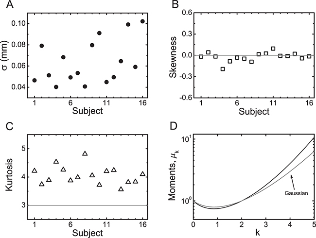
Fig. 2: Statistical aspects of COP velocity series. Values of (A) standard deviation, (B) skewness and (C) kurtosis of the COP velocity for each subject (anteroposterior direction). The dotted lines represent the expected value for a normal distribution. (D) The moments of the standardized COP velocity distribution (black) in comparison with the Gaussian moments (gray).
Download figure:
Standard imageIn order to overcome the variability of the standard deviations, as in the cases of skewness and kurtosis analysis, and to try to identify more patterns related to COP velocities, the following analysis is based on the standardized COP velocity  . In this direction, consider the moments
  of the distribution of standardized COP velocity
  , with
  , where all the series were used as a single normalized data set. Figure 2(D) shows that the moments of the velocity distribution deviate from the Gaussian case as k increases. This result extends the kurtosis analysis for the global data because
  is the kurtosis.
In addition to the above analysis, tests of statistical significance were performed for data of each subject. The null hypothesis that the data is distributed according to the Gaussian distribution is rejected at the 5 percent level based on the Anderson-Darling and Cramér-von Mises tests. This analysis is consistent with previous studies where it was also indicated that COP velocity distributions are significantly different from Gaussians [26,27].
Next, the COP velocity distribution is explicitly calculated, i.e.,  is obtained by using all N = 160 series as a single normalized data set. From fig. 3, one verifies that
  remembers the normal distribution for
  . In contrast, for
  , a deviation from a Gaussian is identified. A direct practical implication of this finding is that large velocities occur with larger probability than expected for a Gaussian process.
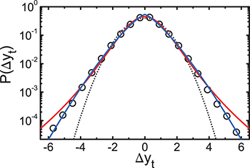
Fig. 3: (Colour on-line) Standardized anteroposterior COP global velocity distribution,  . The dotted line represents a Gaussian with zero mean and unit standard deviation. The continuous lines refer to a q-Gaussian (eq. (3)) with
  (red) and a stretched Gaussian (eq. (4)) where
  (blue), values obtained by using the maximum likelihood estimation.
Download figure:
Standard imageSince COP movements can be viewed as random walks, candidates for COP velocity distributions could be related to Fokker-Planck equations. In the usual case of one-dimensional free-particle motion, the Fokker-Planck equation for the velocity v is given by [29]

where the noise strength D is constant, the friction coefficient γ is also constant and  is the probability velocity distribution at time t. In the stationary case
  , with
  for
for  , this equation reduces to

The solution of this last equation is the Maxwell velocity distribution, i.e., the Gaussian  , with
  being the normalization constant. As the COP velocity distribution exhibits non-Gaussian behavior, candidates for COP velocity distributions (generalized Maxwell velocity distributions) could be investigated from stationary solutions of generalized Fokker-Planck equations. Two cases of generalized Fokker-Planck equations that lead to a significant improvement in the description of the COP velocity distribution, when compared with a Gaussian, are focused here.
As a first generalization, consider  with Dq constant. This leads to a non-linear Fokker-Planck equation [30,31] which recovers the usual one when q = 1. The corresponding solution of eq. (2), when replacing v by
  , is
, is

where Nq is a normalization constant and b is a function of q, Dq and γ. Note that the Gaussian distribution corresponds to  in the limit
  and
and  has fat tails because
  for large
  and q > 1. In addition,
  for
for  . Therefore, eq. (3) has two aspects of COP velocity: a central part resembling a Gaussian and long tails when q > 1.
Equation (3) has been employed in many contexts, from physics and engineering to economics and biology [32,33]. For instance, it was applied with success to model the non-Gaussian velocity distribution of Hydra viridissima cells in two kinds of cellular aggregates [34]. Because the connection of eq. (3) with the Tsallis generalized statistical mechanics, it is usually referred as q-Gaussian. This statistics has been a useful theoretical tool to discuss anomalous behaviors, in particular, when related to non-Gaussians [32,33]. For instance, the usual Maxwell distribution is replaced by eq. (3). In this scenario, many aspects related to the usual (Boltzmann-Gibbs) statistical mechanics have been generalized. An example is the use of the non-linear Fokker-Planck equations [30,31,35,36] replacing the usual ones.
As well as the non-linear Fokker-Planck equation was first introduced in connection with a non-linear anomalous diffusion equation (porous medium equation) [30], another generalized Fokker-Planck equation can be related to other anomalous diffusion. In this direction, the same functional form of Richardson anomalous diffusion equation [37] is employed here but replacing the distance r by the velocity v. This proposal corresponds to using  in eq. (1), with Ds and s being constants. In this case, the solution of eq. (2), a generalized Maxwell distribution, becomes

where v was replaced by  , Ns is a normalization constant and a is a function of s, Ds and γ. Equation (4) reduces to a Gaussian for s = 2 and becomes stretched for s < 2. For this reason, eq. (4) is referred to here as stretched Gaussian. Analogously to the q-Gaussian, the stretched Gaussian is common in many scenarios, such as diffusion in fractals [38], two-dimensional turbulence [39], predator-prey encounters [40], atom deposition into a porous substrate [41], distribution of sound amplitude in music [42], and ergodicity breaking in heterogeneous diffusion processes [43,44].
Since the standard deviation of  is equal to one, standardized q-Gaussian and stretched Gaussian distributions must be employed. As consequence, one has
  , with
  , in eq. (3) as well as
 ![$a= [s\,\Gamma(1+1/s)]^{-s/2}\,\Gamma(3/s)^{s/2}$](https://content.cld.iop.org/journals/0295-5075/109/4/48001/revision1/epl16898ieqn43.gif) in eq. (4), with
in eq. (4), with  being the Gamma function. By using the maximum likelihood method, the COP velocity distribution for our global data was approximated by a q-Gaussian and a stretched Gaussian. Figure 3 suggests that the use of q-Gaussians and stretched Gaussians improves substantially the adjustment of the COP velocities in comparison with a Gaussian.
The same procedure was repeated to analyze the velocity distribution for each subject, i.e.,  , with
  . In this case, as previously pointed out, the ten series for each volunteer were grouped into a series and each
  was approximated by standardized q-Gaussian and stretched Gaussian distributions. An illustration of an individual COP velocity distribution for a representative subject is presented in fig. 4(A). The results of the individual analysis are shown in fig. 4(B) (
 and
and  ), indicating that the q parameter remains larger than 1 and the s parameter is smaller than 2. Moreover, these parameters are close to their global values obtained in the previous analysis,
  and
and  . Tests of statistical significance (Anderson-Darling and Cramér-von Mises tests) indicated that more than 70% (80%) of 160 anteroposterior COP velocity series are not rejected at 1% level for q-Gaussians (stretched Gaussians).
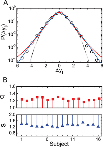
Fig. 4: (Colour on-line) (A) Standardized anteroposterior COP velocity distribution,  , for a representative subject. The dotted line represents a Gaussian with zero mean and unit standard deviation. The continuous lines refer to a q-Gaussian with
  (red) and a stretched Gaussian where
  (blue). (B) Values of the q (top) and s (bottom) parameters obtained for each subject. The solid lines are distances between the experimental values and those obtained from a Gaussian.
Download figure:
Standard imageA similar analysis was performed to the mediolateral direction (left-right movement as Xt in fig. 1(A)). One found  and
and  for the global velocity distribution. For the individual cases,
  and
and  were obtained. The same tests of statistical significance (Anderson-Darling and Cramér-von Mises) pointed out that more than 50% (60%) of 160 velocity series are not rejected at 1% level for q-Gaussians (stretched Gaussians).
In addition to the analysis of COP velocity distributions, we present below results concerning COP position distributions. Following a similar procedure to the velocity series, the fitting parameters obtained for the global position distribution were q close to 1 when employing q-Gaussians and s close to 2 for stretched Gaussians for both directions, anteroposterior (AP) and mediolateral (ML) ones. Explicitly, these values were  and
and  for AP (ML). Skewness in both directions was near to zero,
  , and kurtosis 3.02 (3.22) for AP (ML) direction. For each individual, the values of q, s, skewness and kurtosis remained close to the global values. For the tests of statistical significance (Anderson-Darling and Cramér-von Mises) less than 18% (22%) of 160 position series were not rejected at 1% level for q-Gaussians (stretched Gaussians) in both directions. These results show that the non-Gaussian behavior for the position series is subtle or almost imperceptible.
To conclude our discussion about COP velocity distribution, the main achievements are summarized and possible implications of our findings are raised. Consistently with the literature [28], fig. 2(A) indicated that standard deviations exhibit large variability from a subject to another and therefore cannot be used as a typical characteristic of all subjects. To investigate more deeply aspects unrelated to the standard deviation, a standardized COP velocity was employed here. In contrast to the investigation of standard deviations, the skewness analysis (fig. 2(B)) pointed out in the direction that COP velocity distributions are well approximated by symmetric ones. In addition to this common aspect for all subjects of our analysis, the kurtosis values indicated a robust fat-tail pattern for COP velocity distributions when compared with a Gaussian (fig. 2(C)) and reinforced by a moment study (fig. 2(D)). The non-Gaussian profile was also verified by tests to decide if the velocity data comes from a Gaussian distribution, consistently with previous studies [26,27]. In addition, for standardized velocities, very similar distributions were identified for all subjects. And, considering generalized Fokker-Planck equations for COP velocities, the non-Gaussians distributions with fat tails can be interpreted as generalized Maxwell velocity distributions. These distributions were well approximated by q-Gaussians and by stretched Gaussians (figs. 3 and 4).
The empirical results obtained here for COP velocity distributions, together with those about correlations [19–21,24], compose a useful guide to model COP dynamics. However, others studies are still required to obtain a broader scenario for COP velocity distributions. Future works could investigate the sensitivity of COP velocity distributions to changes in postural steadiness related to age, neurological and orthopedic diseases or other pathologies affecting the postural control system.
Concerning the models employed here, they represent a first view of the scenario of COP velocities. In the model related to q-Gaussians, the noise strength D is proportional to a negative power of the probability distribution,  with q > 1, leading a non-linear stochastic process. For the case of stretched Gaussians, the noise strength is proportional to
  with s < 2, that is, a heterogeneous model. If one is interested in a model that accommodates q-Gaussians and stretched Gaussians in a unified way [45],
  could be used. Another possibility would be to consider other models that have stretched Gaussians as solutions. This is the case of the fractional Fokker-Planck equation [46,47], which is equivalent to continuous time random walk models with scale-free waiting times. Such a model presents a degree of memory and could be useful in connection with some regulatory mechanism in the maintenance of the upright standing. In turn, this Fokker-Planck equation and heterogeneous models exhibit weak non-ergodic behavior [43,44,48]. Motivated by a possible connection between these models and COP dynamics, the time dependence of the mean square displacement, measured from single COP trajectories, could be investigated. This procedure would give direct experimental verification of an anomalous stochastic process and of a non-ergodic character. Furthermore, to employ this procedure is useful because probability distributions could not be the best way to identify anomalous stochastic processes. All these aspects illustrate possible perspectives for further analysis involving upright quiet stance data.
Acknowledgments
This research was supported by the Brazilian agencies Conselho Nacional de Desenvolvimento Científico e Tecnológico (CNPq) and Coordenação de Aperfeiçoamento de Pessoal de Nível Superior (CAPES).