


Abstract
It is shown that there is a linear relation between the relative Rényi entropy and the density functional fidelity susceptibility. The derivative of the relative Rényi entropy with respect to the Rényi parameter α is also proportional to the density functional fidelity susceptibility. The benefit of these relations is illustrated for the Dicke model (considering a numerical study and a variational analytical approximation). These relations are useful to detect the second-order QPT in this model.
Export citation and abstract BibTeX RIS
There has been a growing attention to information theoretical concepts, in particular, Shannon [1], Fisher [2] and Rényi [3] information has been proved to be very useful in several fields of physics, e.g. in the analysis of quantum entanglement [4], quantum communication protocols [5], quantum correlations [6], quantum revivals [7,8], localization properties [9]; in analyzing atomic and molecular properties [10–27] or in studying quantum phase transitions (QPTs) [28–34].
QPT is an extension of the concept of classical phase transition to quantum systems at zero temperature [35], where quantum fluctuations are responsible for a dramatic change in the system properties. QPTs have recently been considered from a density functional theory (DFT) aspect [36–38]. DFT is frequently applied nowadays to obtain the energy levels of systems. It can, of course, be used to study QPT. In DFT the density is the basic variable that determines all properties of many-particle systems. In the DFT visualization of QPT an analogue of the DFT density is introduced. This new "density" determines the control parameter(s), that corresponds to the DFT "external potential" [36]. In a non-degenerate ground state, there is a bijective map between the density and the control parameter(s). Moreover, any strictly monotonous function of the "external potential" leads to a new "density" with a different control parameter, which is determined by the new "density". There is also a one-to-one map between the Rényi entropy of a given order and the control parameter. Therefore, the Rényi entropy can be used as a control parameter [37]. (Degenerate cases can be similarly treated utilyzing the so-called "subspace density" [38].) Because of this important role of the Rényi entropy, we explore the link between the relative Rényi entropy [39] and the fidelity susceptibility. It is a generalization of our recent work on the approximate proportionality of the density functional fidelity susceptibility and the relative or Kullback-Leibler entropy [40]. Now, we prove that the relative Rényi entropy is approximately proportional to the fidelity susceptibility and the relative Rényi entropy is the Kullback-Leibler entropy multiplied by the Rényi parameter. The usefulness of these concepts is explored in the context of QPTs. We mention in passing that the Kullback-Leibler entropy has recently been used to quantify chemical reactivity [41,42].
Consider a distribution function f. The Rényi entropy of order α is defined as [3]

The limit  gives the Shannon entropy:

The relative Rényi entropy of order α is defined as a measure of the deviation of  from a reference density
  as [3]

provided that the integral on the right exists and  . The limit
  gives the relative or Kullback-Leibler entropy (also called cross-entropy) [43]

which is a particular measure of the deviation of  from
from  .
.
On the other hand, quantum fidelity [44] is defined by the overlap between the states  and
and  as
as

for pure states. There is an analogous definition in the density functional theory [45],

It gives the deviation of two states characterized by the densities ϱ and σ. The density ϱ (or σ) is given by

In case of a many-variable wave function,

is a reduced density (q and τ can denote several variables). Obviously, several reduced densities can be constructed for a many-variable wave function. Since fidelity is a measure of similarity between states, that can also been described by the relative Rényi entropy, there should be a relationship between these quantities.
Consider a system in which there is a QPT. The Hamiltonian can be written as  , so it is governed by a control parameter λ. At the critical point
  , there is an abrupt change in the symmetry of the ground-state wave function. The fidelity can be determined at two close points λ and
  . Then we expand the fidelity around λ

where  is the fidelity susceptibility [45]. Similarly, the expansion of the density functional fidelity

leads to the density functional fidelity susceptibility 
On the other hand,  is proportional to the Fisher information [2]

(It can be easily shown if we expand  around
  in eq. (6).) The Fisher information provides a measure to estimate the parameter λ. We mention in passing that if λ is a parameter of locality, that is,
  , eq. (12) does not depend on λ [12]. Then the Fisher information can be rewritten as
However, eq. (12) generally differs from eq. (13). In this paper the general form (eq. (12)) is applied.
Now we derive the relationship between the relative Rényi entropy of order α and the fidelity susceptibility. Expanding  around
  we are led to
Multiplying with  and integrating we obtain
The integral of the first and second derivative of  with respect to λ disappears, because

The first-order term disappears and the second-order term (which remained) is proportional to the Fisher information (12),

Then the relative Rényi entropy of order α (3) can be written as

and for small x we can use the expansion  , therefore

Note that if  , eq. (19) reduces to the relative or Kullback-Leibler entropy:

Numerical results below show that expression (19) is better if the value of α is larger. Therefore, it is worth using the relative Rényi entropy instead of the Kullback-Leibler entropy. Note that the relative Rényi entropy of order α is the Kullback-Leibler entropy multiplied by the Rényi parameter α:

This is an amazingly simple relation. It is the obvious consequence of the fact that two close points with λ and  are considered. Density functional fidelity is in a linear relationship with the relative Rényi entropy:

This approximation will be very good except around a region at the critical point, where I could be large. We can define

to measure the quality of (22), which will be 1 except around the critical point. Another important expression is obtained by taking the derivative of the relative Rényi entropy with respect to α,
To illustrate the advantage of the relation between the fidelity and the relative Rényi information we consider the Dicke model which is a representative model of spin-boson interactions. This model has been used in the study of quantum optical, chaotic and entanglement properties (see [46–52]). It is important to point out that recently, some experiments have provided a direct realization of the Dicke model [53,54].
The Dicke model [46,50–52] describes an ensemble of N two-level atoms, with level splitting  , interacting with an electromagnetic field with frequency ω and with a coupling parameter λ for the dipolar interaction between the field and the atoms. If we use the a and
  bosonic operators of the field, the Hamiltonian is given by

where Jz,  are the angular momentum operators for a pseudospin of length
  . It has been proved that there is a quantum phase transition for
  in the thermodynamic limit
  , and there are two phases: for
  and for
  , the so-called normal and superradiant phases, respectively. The system has the parity symmetry, that is, the parity operator
  , which verifies
 ![$[\hat\Pi,H]=0$](https://content.cld.iop.org/journals/0295-5075/109/6/60002/revision1/epl16968ieqn33.gif) .
.
A basis set of the Hilbert space is  , with
  the number states of the field and
  the so-called Dicke states of the atomic sector, so we can express a general vector ψ of the Hilbert space as the expansion
where the coefficients  have been determined numerically. For this purpose we have truncated the bosonic Hilbert space, taking into account the first nc states of the field in the basis set.
Now we can write the position density as

where  is the position space wave function:
where we have used the position representation of the field sector:
and the Holstein-Primakoff approximation (see [55]) to represent in position space the atomic sector

In figs. 1 and 2 we plot the quantity  for
for  and 1/2, respectively, as a function of λ for j = 3, 5 and 10. We have taken
  in all the cases. We can observe that the approximation of
  by 1 is really good for all the values of the parameter λ, but it is clear that the approximation in eq. (23) is better as λ is further from the critical point
  . On the other hand, it is apparent in both figures that the difference of
  from 1 around the critical point is sharper as the j value increases. In fig. 3 we have plotted the quantity
  as a function of λ for j = 3, 5 and 10, to check the linear relationship obtained in eq. (22). Again we can see that the approximation is very good, but it is better as λ is further from the critical point. Note that expression (19) is a better approximation for larger values of α.

Fig. 1: (Colour on-line)  for
for  for j = 3, 5 and 10 and
  in terms of λ for the numerical ground-state wave function. Atomic units are used.
Download figure:
Standard image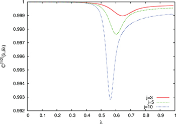
Fig. 2: (Colour on-line)  for
for  and for j = 3, 5 and 10 and
  in terms of λ for the numerical ground-state wave function. Atomic units are used.
Download figure:
Standard image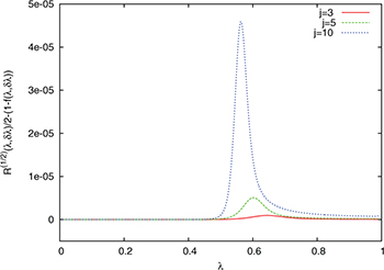
Fig. 3: (Colour on-line)  for
for  and for j = 3, 5 and 10 and
  in terms of λ for the numerical ground-state wave function. Atomic units are used.
Download figure:
Standard imageFor completeness we will do an analytical variational approximation analysis of the ground state of the Dicke model. We will use the variational approximation introduced by Castaños et al. [56,57] which takes into account the Hamiltonian parity symmetry
with the normalization factor
where the variational parameters α and z can be computed minimizing the mean energy and are given by (see, for example, [28,32–34])
and where the Holstein-Primakoff approximation (see [28,32] for details) has been used.
In fig. 4 we present  for the variational approximation, for
 ![$\lambda\in[0,1]$](https://content.cld.iop.org/journals/0295-5075/109/6/60002/revision1/epl16968ieqn60.gif) and for j = 3, 5 and 10. We have taken
and for j = 3, 5 and 10. We have taken  . The variational approximation value of
  is around 1 and again this approximation is better as λ values are further from the critical point
  .
.
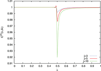
Fig. 4: (Colour on-line)  for
for  and for j = 3, 5 and 10 and
  in terms of λ for the ground-state variational approximation. Atomic units are used.
Download figure:
Standard imageIn summary, if we consider QPTs from a DFT aspect, we have demonstrated that there is a linear relation between the relative Rényi entropy (and also between the derivative of the relative Rényi entropy with respect to the Rényi parameter α) and the density functional fidelity susceptibility. The advantage of these relations is illustrated by a numerical study and a variational analytical approximation of the Dicke model, in which there is a second-order QPT for a critical value  of the coupling parameter λ (which quantifies the dipolar interaction between the field and the atoms). We have verified that the approximation is very good for all the values of the parameter λ except in a region around the critical point
  , so it is shown that the presented relations are useful to detect the second-order QPT in this model.
Acknowledgments
The work is supported by the TAMOP 4.2.2.A-11/1/KONV-2012-0036 project. The project is co-financed by the European Union and the European Social Fund. Grant OTKA No. K 100590 is also gratefully acknowledged. The work is also supported by the Spanish Projects CEIBIOTIC-UGR PV8, the Junta de Andalucía projects FQM.1861 and FQM-381.