


Abstract
The emergence of ferroelectricity in nanotubes and spherical nanoshells is studied theoretically. We determine semi-analytically the size and thickness dependence of the ferroelectric instability, as well as its dependence on the properties of the surrounding media and the corresponding interfaces. By properly tuning these factors, we demonstrate possible routes for enhancing the ferroelectric transition temperature and promoting the competition between irrotational and vortex-like states in the ultra-thin limit due to the specific topology of these nanoparticles.
Export citation and abstract BibTeX RIS
Ferroelectric nanoparticles receive a considerable research attention [1–13] and novel fabrication methods are being developed [14,15]. The case of ferroelectric nanotubes and nanoshells is particularly interesting, as their specific topology can be exploited for engineering additional functionalities relevant for technological applications [1,2,16]. However, one of the limiting factors of these systems is the ferroelectric instability itself, as the corresponding transition temperature Tc can drop drastically due to finite-size effects [7,17–24]. In this paper we address this crucial point within the Ginzburg-Landau-like formalism, with which we describe analytically the ferroelectric transition in nanotube and nanoshell geometries. Thus, we extend the considerations reported in [4,5,7,8,12,25,26] to novel geometries of experimental relevance. Specifically, in the case of ferroelectric nanotubes, we will consider the electric polarization perpendicular to their axis. In addition to the overall size effect, we analyse the impact of the thickness, relative permittivities, and boundary conditions on the possible competition between different type of polarization distributions.
The emergence of ferroelectricity in a finite-size system is ultimately determined by two fundamental factors [21,27]. On the one hand, there is the tendency towards ferroelectricity itself, which can satisfactorily be modelled within the Ginzburg-Landau formalism [21]. This provides the constitutive equation in the ferroelectric that, to our purposes, can be linearised and taken as  , where P is the ferroelectric polarization and Φ is the electric potential. Here
  is the inverse susceptibility, with Tc0 being the nominal transition temperature
  , and g is associated to the gradient term in free energy. For the sake of simplicity, the response of the ferroelectric is assumed to be isotropic —either completely (nanoshell) or within the ferroelectric plane (nanotube). As in [7,12], this approximation is expected to capture the key qualitative features of the ferroelectric instability1
. On the other hand, there is a purely electrostatic aspect described by Gauss's law:
, and g is associated to the gradient term in free energy. For the sake of simplicity, the response of the ferroelectric is assumed to be isotropic —either completely (nanoshell) or within the ferroelectric plane (nanotube). As in [7,12], this approximation is expected to capture the key qualitative features of the ferroelectric instability1
. On the other hand, there is a purely electrostatic aspect described by Gauss's law:  , where ε is the so-called background permittivity [28], and the corresponding boundary conditions [21,27]. Thus, whenever
  , the spontaneous polarization will be penalised by the accompanying electric potential and the corresponding increase of electrostatic energy.
Following [7], the task is to find the nontrivial solution of the above equations that can appear at the highest T (i.e., for the maximum value of the coefficient a). This search can be restricted to the family of divergenceless distributions of polarization  that automatically minimize (most of) the electrostatic energy in the ferroelectric. Furthermore, two subfamilies can be identified among the targeted distributions: i) irrotational distributions
  and ii) vortex-like states
  . In the first case the gradient energy is minimised at the expense of some electrostatic energy generated by interfacial bound charges (depolarizing field). In the second case the situation is reversed, and the electrostatic energy is minimised at the expense of some gradient energy in the ferroelectric. These cases will be analysed separately for the different geometries of interest, and the results will be illustrated by considering the material parameters of BaTiO3.
In the case of a cylinder or a sphere, the only possible irrotational distribution of polarization corresponds to the  (homogeneous polarization). The presence of the internal boundary in the nanotube or the nanoshell, however, introduces more complex patterns. In this case, since
  , the above equations reduce to the Laplace equation
  . We thus adopt cylindrical
  and spherical
  coordinates for the nanotube and the nanoshell, respectively, and consider the solutions


for the electrostatic potential, where  represent the Legendre polynomials. Hereafter
  represents the internal (external) radius. The irrotational distributions of polarization are illustrated in fig. 1. n = 1 corresponds to the homogeneous polarization for
  (see fig. 1(a)). Whenever
  , however, the resulting polarization is inhomogeneous (fig. 1(b)), and this inhomogeneity increases with the corresponding order n (fig. 1(c)).

Fig. 1: (Colour online) Irrotational distributions of polarization (a)–(c) and vortex-like polarization (d) across the cross-section of a ferroelectric nanotube. (a) and (b) correspond to n = 1, while (c) to n = 3.
Download figure:
Standard imageWe consider first the (2D) case of a nanotube. The electric potential Φ has to be continuous at R1 and R2, while its gradient has to be such that  . Here n is the normal unit vector to the interface while
  represents the interfacial charge density. In order to ensure charge neutrality, the interfacial charge densities can be taken as
  and
and  , with P0 being a constant. Thus, the solutions (1) become compatible with the boundary conditions whenever the condition

is satisfied. Here  is the permittivity of the ferroelectric, while
  and
and  are those of the inner and outer medium, respectively. Equation (3) determines the hypothetical Tc associated to the irrotational solutions (1) as a function of
  and the corresponding order n, which is illustrated in fig. 2. As we can see, while all orders tend to be degenerate in the limits
  and
and  , the highest Tc corresponds to the n = 1 solution and this hierarchy is maintained for all the radii
  .
.

Fig. 2: (Colour online) Tc associated to irrotational distributions of polarization in ferroelectric nanotubes.  ,
,  ,
,  and
and  .
.
Download figure:
Standard imageIn the (3D) case of the nanoshell, the interfacial charge densities can be taken as  and
and  . Thus, the compatibility between the solutions (2) and the electrostatic boundary conditions implies
We now have two different situations depending on the relative permittivities  and
and  . If
. If  (see fig. 3(a)) the degeneracy at
  is lifted, although the n = 1 solution has always the highest Tc as in the previous (2D) case. If
  (see fig. 3(b)), however, this hierarchy is reversed for small R1 and, interestingly, a crossover is obtained as the
  ratio increases.

Fig. 3: (Colour online) The relation between  and
and  with respect to different orders of the FE nanoshell structure. (a)
  and
and  , while for (b)
  and
and  , other parameters are the same as for the nanotube.
Download figure:
Standard imageInterestingly, in both 2D and 3D cases, the strong suppression of the Tc of the irrotational polarization can be moderated in the limit  . However, the question of whether they can be realised experimentally eventually depends on the competition with other families of solutions. In the following we consider the vortex-like patterns, as they are the most serious contenders.
In our systems, a vortex-like distribution of polarization implies  everywhere, and hence
  . Thus, the emergence of this type of polarization is simply governed by the equation
  under the corresponding boundary conditions. The solutions of interest can be written as
  , where


for the (2D) nanotube and (3D) nanoshell geometries, respectively. Here  is the correlation length, J1 and Y1 are Bessel functions of first and second kind, while j1 and y1 are spherical Bessel functions of first and second kind, respectively.
The Tc associated to these vortex-like distributions of polarization depends on the boundary conditions. We consider the general boundary conditions  , where λ is the so-called extrapolation length [21]. Thus, in the (2D) case of a nanotube Tc is determined by
A similar equation is obtained for the (3D) nanoshell case with  . For the sake of simplicity, we consider that the two interfaces are described by the same λ (see footnote 2
).
. For the sake of simplicity, we consider that the two interfaces are described by the same λ (see footnote 2
).
We find that the Tc as a function of R1 and R2 can show rather different behaviors when these parameters are varied separately. This is eventually determined by the extrapolation length λ, as illustrated in fig. 4 for the case of a ferroelectric nanotube. Specifically, the "topography" of the  map changes in such a way that its maximum gradient rotates by 45° as λ goes from 0 to ∞. Thus, for
  , Tc decreases by decreasing the thickness of the shell. That is, by either increasing R1 or decreasing R2 (A-O and B-O paths, respectively, in fig. 4(a), which correspond to blue and orange lines in the bottom plot). For a finite λ (fig. 4(b), (c)), however, Tc initially increases by increasing R1 and then decreases after reaching a maximum. By decreasing R2, in contrast, the behavior is monotonous and Tc always decreases. For
  , which corresponds to the so-called natural boundary conditions
  , the dependency on the nanotube thickness is different for different paths (fig. 4(d)). While Tc increases by increasing R1, it decreases by decreasing R2. This unequivalence in the finite-size effect is related to the specific topology of the systems under consideration. In fact, in the case of the nanoshell, the Tc associated to the vortex-like distribution of polarization behaves qualitatively in the same way within the approximations of our model.
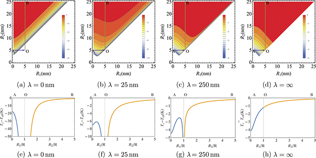
Fig. 4: (Colour online) Transition temperature for a vortex-like polarization state in a ferroelectric nanotube  . Top: contour plots for
  as a function of the internal
  and external
  radii of the nanotube. Bottom:
  along the paths A-O (blue) and B-O (orange).
Download figure:
Standard imageWe note that, compared to the irrotational states, the Tc associated to vortex-like distributions of polarization is generally much closer to its nominal value Tc0 (irrespective of the properties of the surrounding media). However, when  , the Tc for the vortices can drop significantly while that of the irrotational distributions approaches Tc0. Thus, we find that the specific topology of these systems enables the competition between different type of polarization distributions in the ultra-thin limit.
In summary, we have studied theoretically the ferroelectric instability in nanotubes and spherical nanoshells. Specifically, we have considered semi-analytically different families of polarization distributions and examined how their emergence is affected by the thickness of the nanoparticle, the dielectric properties of the surrounding media, and the interfacial boundary conditions. We have found an intriguing topological finite-size effect that can promote the competition between different types of ferroelectricity in the ultra-thin limit. These results illustrate new routes to control the ferroelectric instability and engineer ferroelectric properties at the nanoscale. This possibility is expected to motivate both extended theoretical analyses and future experimental work.
Footnotes
- 1
A more realistic description including, e.g., strain fields is beyond the scope of this inaugural work.
- 2
Qualitatively, the same results are obtained for different extrapolation lengths.