Abstract
We derive the magnetization of a system, Pierre Curie's law, for paramagnetic particles out of thermal equilibrium described by kappa distributions. The analysis uses the theory and formulation of the kappa distributions that describe particle systems with a non-zero potential energy. Among other results, emphasis is placed on the effect of kappa distribution on the phenomenon of having strong magnetization at high temperatures. At thermal equilibrium, high temperature leads to weak magnetization. Out of thermal equilibrium, however, strong magnetization at high temperatures is rather possible, if the paramagnetic particle systems reside far from thermal equilibrium, i.e., at small values of kappa. The application of the theory to the space plasma at the outer boundaries of our heliosphere, the inner heliosheath, leads to an estimation of the ion magnetic moment for this space plasma, that is,  .
.
Export citation and abstract BibTeX RIS
Introduction
Classical particle systems reside at thermal equilibrium with their velocity distribution function stabilized into a Maxwell distribution. On the contrary, collisionless and correlated particle systems, such as the space and astrophysical plasmas, are out of thermal equilibrium and characterized by a non-Maxwellian behavior, typically described by the so-called kappa distributions. Indeed, these distributions (single types or combinations thereof) have been used to describe ion-electron populations in space plasmas throughout the heliosphere, from the solar wind and planetary magnetospheres to the inner heliosheath and beyond (see [1] and references therein).
Since their introduction in space physics about half a century ago [2,3], empirical kappa distributions become increasingly widespread across space and plasma physics. These distributions were exhaustively used to study the statistical behaviour of particle kinetic energy in the absence of any potential energy. However, an important development in the field came with the connection of kappa distributions to the statistical framework of non-extensive statistical mechanics [4]. Understanding the origin of kappa distributions was the cornerstone of important theoretical developments and applications.
One of these developments was the derivation of the phase-space kappa distribution of a Hamiltonian with a non-zero potential [5]. Particle systems described by kappa distributions, such as space plasmas, are typically characterized by various short- and long-range interactions, where both the kinetic and the potential particle energies must be taken into consideration in the statistical description. The statistical analysis of a system of paramagnetic particles is such an example.
Non-extensive statistical mechanics, in brief
Non-extensive statistical mechanics was introduced in [6] as a possible generalization of the classical framework of Boltzmann-Gibbs statistical mechanics. The main suggestion was to generalize the formulation of entropy, depending on a parameter, q. The maximization of this new type of entropy under the constraint of fixed internal energy leads to the probability distribution of energy within the framework of canonical ensemble. The characteristic exponent of the canonical distribution was  and it has been connected with a type of kappa distributions under the transformation
  [7]. However, the earliest non-extensive statistical mechanics was suffering from some fundamental issues. In particular, the canonical distribution of energy was not invariant under arbitrary selections of the zero-level energy, while the internal energy was not extensive as it should be for uncorrelated distributions. These two inconsistencies as well as various other problems were finally solved a decade later in [8]. Thereafter, the characteristic exponent of the canonical distribution is
  , which is connected with the primary type of kappa distributions under the transformation
  [9].
[9].
There are several differences between the structures of the old and the modern non-extensive statistical mechanics. The latter generalizes the notion of the canonical distribution via the formalism of escort probabilities. The ordinary  and escort
  probability distributions [10] are related

Most important, modern non-extensive statistical mechanics canonical distribution includes correctly the notion of temperature. The temperature acquires a physical meaning as soon as Maxwell's kinetic definition [11] coincides with Clausius's thermodynamic definition [12]. The latter was modified by [13] using the "physical temperature", in order to be aligned with the zeroth law of thermodynamics [14]. This is the actual temperature of a system; it is unique and independent of the q or κ indices. (For more details, see [1,9,14,15].)
In short, these are the advantages of the modern non-extensive statistical mechanics, as opposed to its earliest version: i) Independence of the zero energy level. ii) Consistent partition of the system's internal energy to the subsystems' partial internal energies. iii) Physically meaningful temperature.
In the earliest version, the formulation of the canonical distribution using q or κ indices, was

On the other hand, in the modern version the distribution is

where  is the ensemble phase-space average of the Hamiltonian function. In the absence of potential, (3) becomes
where we substituted the mean kinetic energy with  . Moreover, the kappa index κ depends on the particle kinetic degrees of freedom
  , i.e.,
  . The quantity κ0 indicates the kappa index which is independent of the degrees of freedom [16–18]. The kappa distribution in (4) may be rewritten in terms of the invariant kappa index, κ0,

Effects of the kappa distribution on the Curie law
Let us consider a system of paramagnetic particles with freely rotating magnetic moments  in the presence of an external magnetic field
  . Setting the z-axis on the direction of
  , the particle potential energy is given by

where ϑ is the polar angle between the external magnetic field vector and the magnetic momentum vector of each particle;  is set to be aligned with the field with unit vector
  , so that
  .
.
The magnetization M of a paramagnetic material is proportional to the strength B of an external magnetic field and inversely proportional to the temperature T, in the approximation of high temperature, that is,  (small magnetic energy over large thermal energy). This behavior constitutes Curie's law, which is expressed using the Curie constant C as the proportionality coefficient

The per particle magnetization is given by the average magnetic moment,  , the total magnetization is
  (for N particles), while the magnetization density is given by
  (for number density n). Given
  ,
,  is determined using the positional probability distribution

where  , and
, and  abbreviates the dependence on the solid angle. If there is no radial dependence, then the distribution becomes angular, while if there is also no dependence on the azimuth φ but only on the polar angle ϑ, then the angular distribution becomes
  , and
, and  is (where
  because of azimuthal symmetry)

The classical phase-space distribution function is constructed by the Boltzmann-Gibbs energy distribution, with the energy substituted by the Hamiltonian function

Within the theory of kappa distributions [1,9,15] and its statistical framework of non-extensive statistical mechanics [4,6,8,19] and superstatistics [20–24], eq. (10) becomes the kappa distribution of the Hamiltonian [5],

In terms of the invariant kappa index κ0, (11) becomes

or, in terms of the kinetic energy,  ,
,

with normalization and positional probability distribution

The analytical derivations of the kappa distributions of the phase-space ( and
and  ) was shown in [5],

with marginal distributions

and

The mean  is implicitly given by

This can be also expressed through a generalization of the Langevin function, i.e.,
and the per particle magnetization  becomes
(plotted in fig. 1). The q-Langevin function is defined as

recovering the standard Langevin function for  or
or  ,
,  . It employed the q-hyperbolic cotangent,
using the q-exponential (in terms of q or κ0)

(The subscript + notes the cut-off condition ![$[y]_{+} =y$](https://content.cld.iop.org/journals/0295-5075/113/1/10003/revision1/epl17604ieqn41.gif) if
if  and
and ![$[y]_{+} =0$](https://content.cld.iop.org/journals/0295-5075/113/1/10003/revision1/epl17604ieqn43.gif) if
if  .) The q-exponential function has been used in numerous studies related to the non-extensive statistical mechanics [4]. This is mostly known as the q-deformed exponential function [25,26], while the q-deformed hyperbolic trigonometric functions have been developed in [27].
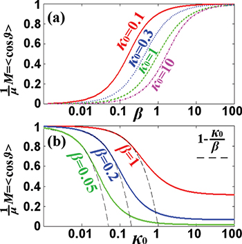
Fig. 1: Magnetization depicted as a function of (a) the inverse temperature,  , and (b) the invariant kappa index, κ0, where the limiting behavior
  is also shown (black dash). We observe that the magnetization tends to zero either for high temperatures (small β) or for large kappa index κ0. On the contrary, the magnetization tends to its largest value either for low temperatures (large β) or for small κ0. Hence, both temperature T and kappa κ0 have the same impact, that is, negative correlation with magnetization. Strong high-temperature magnetization can be realized in systems far from thermal equilibrium
  .
.
Download figure:
Standard imageThe Taylor expansion of the q-Langevin function is  or
or  . This leads to the one-particle magnetization equation,

hence, the Curie constant is kappa dependent,

and the paramagnetic susceptibility becomes

Note that the expansion for higher terms gives

(The 2nd-order term is zero for any κ, thus the 1st-order expansion is a good approximation.)
The phenomenon of paramagnetism has been studied in the framework of non-extensive statistical mechanics [28,29]. In these studies, the earliest version of non-extensive statistical mechanics was used. As explained in the second section, this version used the ordinary probability distribution function with exponent  , instead of the escort probability with exponent
  [9]. Also, the old version does not use the notion of physical temperature which is aligned with the zeroth law of thermodynamics, and is characterized by the equivalence between thermodynamic and kinetic temperature definitions [1,9,14,15,30] (see also [31]). In contrast, the modern non-extensive statistical mechanics is based on the standard Tsallis entropy [6] and the escort probabilities [8], and uses the physical temperature as the actual temperature of the system. Finally, the modern theory takes into account the dependence of q and
  indices on the degrees of freedom
  (as was shown by [16,17]).
Application to the plasma in the outer heliosphere
The presented theory is applied to the proton plasma in the inner heliosheath, the outer boundary of our heliosphere. By fitting kappa distributions to the proton energy distributions, Livadiotis et al. [32] derived the sky maps of the radially averaged values of several thermodynamic quantities in the inner heliosheath, such as, the number density n, the temperature T, and the kappa indices κ. The magnetic field B values have been estimated in [33], using the theory of large-scale quantization that relates B with other plasma parameters.
Having the values of  distributed over the inner heliosheath, it is straightforward to derive the (per particle) magnetization
  . For this reason, we construct the following datasets: i) The magnetization dataset
 ![$M_{i} (\alpha)/\mu \equiv f\,[\beta_{i} (\alpha),\kappa_{0i}]$](https://content.cld.iop.org/journals/0295-5075/113/1/10003/revision1/epl17604ieqn67.gif) , expressed as a function of the unknown parameter α that we wish to estimate; it is defined via the parameter β as follows:
, expressed as a function of the unknown parameter α that we wish to estimate; it is defined via the parameter β as follows:  , i.e.,
  ; and ii) the inverse beta-plasma dataset
  (where beta-plasma
  is the ratio of thermal over magnetic pressure). The parameter α is related to the magnetic moment, thus, once we estimate α, automatically we also derive μ. The magnetization is expected to have a positive correlation with the magnetic pressure and negative correlation with the thermal pressure; hence, a positive correlation should exist between the datasets of the magnetization
  and the inverse plasma beta
  .
.
In fig. 2(a) the magnetization  is plotted as a function of
  . Panel (b) shows the histogram of the magnetization values. We then seek for the highest correlation R between the pair of datasets
  , with
  . In panel (c), the modified correlation
  is plotted, which helps to estimate the uncertainty of α, according to the technique in [34] (for example, applying the method of correlation maximization to the data derived from [32,35], the analysis in [34] found the polytropic index in the inner heliosheath to be close to zero.) The parabolic behavior near the minimum
  of
of  , is expressed by
  , with
  ,
,  ,
,  . The error is
 ![$\delta \alpha_{0} \cong \sqrt {A_{0} /[(N_{0} -1)A_{2}]}$](https://content.cld.iop.org/journals/0295-5075/113/1/10003/revision1/epl17604ieqn85.gif) , where
, where  is the number of data points (which are confident when
  [32]); then we find
  . Therefore, we estimate the magnetic moment of the space plasma ions in the inner heliosheath to be
  . (This is in good agreement with the magnetic moment
  that was found for the Earth's plasma sheet and magnetotail [1], also coincides with the average electron magnetic moment found by [36].)
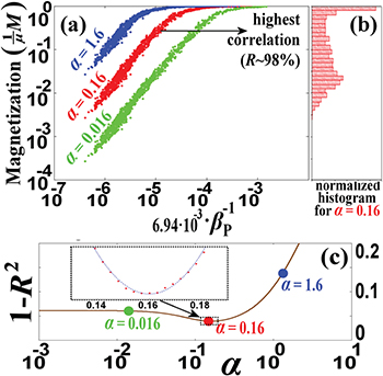
Fig. 2: (a) Magnetization  plotted as a function of the inverse beta-plasma,
  , of the proton plasma in the inner heliosheath. The magnetization depends on the auxiliary parameter
  , defined by
  . Three values of α are examined: i)
  (blue), ii)
  (red), and iii)
  (green) (the datasets
  are taken from [32,33]). (b) Normalized histogram, revealing the most frequent values
  and
and  . (c) The correlation R between the two examined datasets
 ![$M_{i}(\alpha)/\mu \equiv f[\beta_{i} (\alpha ), \kappa_{0i}]$](https://content.cld.iop.org/journals/0295-5075/113/1/10003/revision1/epl17604ieqn61.gif) and
and  is estimated as a function of α, maximized for
  ; the plotted
  helps to estimate the uncertainty of α [34].
Download figure:
Standard imageDiscussion
We have seen that the standard Langevin function at thermal equilibrium is recovered for  or
or  . At the furthest stationary state from equilibrium,
  or
or  , Langevin function behaves asymptotically with a logarithmic divergence. However, the condition for eq. (22) to be valid is
  [5]. Therefore, the furthest possible stationary state corresponds to the kappa value
  that satisfies the relation
 ![$\kappa_{0\min}=\beta \cdot [1-f(\beta,\kappa_{0\min})]$](https://content.cld.iop.org/journals/0295-5075/113/1/10003/revision1/epl17604ieqn97.gif) , where f denotes the function
, where f denotes the function  implicitly expressed by eq. (22) and plotted in fig. 1.
Next, we show that  : We write
  , with
  , so that
  . Hence, as
  , we have
  , thus, the relation
 ![$\kappa_{0} =\beta \cdot [1-f(\beta,\kappa_{0})]$](https://content.cld.iop.org/journals/0295-5075/113/1/10003/revision1/epl17604ieqn105.gif) is defined for any
is defined for any  , thus
  . Therefore, the assumption
  , that is,
  is true; in other words, for small values of kappa,
  , the lower limit of the magnetization
  is
is  , so that
  when
when  .
.
Therefore, we construct the magnetization for the extreme stationary states at thermal equilibrium  and anti-equilibrium (the special state that is furthest from thermal equilibrium,
  , see [1,7,17]):
The importance of the dependence of the Curie constant on the kappa index is that it can create high values of this constant even in the high-temperature environment. Therefore, a strong magnetization of paramagnetic particles is possible at high temperatures when the system resides far from thermal equilibrium (low values of κ0). As is observed, the Curie constant C depends on the kappa index; it is monotonically decreasing with κ0, i.e., lower values of the kappa index lead to larger values of the Curie constant. We notice that  , for small values of
  , hence, if
  , then,
  . Thus, the low-temperature magnetization that appears for
  and near-equilibrium
  , can show up at higher temperatures, e.g.,
  and far from equilibrium, i.e.,
  . We also remark that the magnetization density behaves like
  , while the dependence of the Debye length on the kappa index is
  [37–40]. Hence, the magnetization density per magnetic field depends only on the Debye length,
 ![$[M_{\text{V}}/(\mu^{2}\,B)]\cdot \lambda_{\text{D}}^{2}\cong\textstyle{1 \over 3}\varepsilon_{0} e^{-2} \cong 1.15\times 10^{26}\ \text{J}\cdot \text{m}$](https://content.cld.iop.org/journals/0295-5075/113/1/10003/revision1/epl17604ieqn127.gif) .
.
Finally, the main conclusions and findings of this work are:
- The equation of magnetization uses the q-Langevin function with
 . The standard Langevin function at thermal equilibrium is recovered for or , while at the furthest stationary state from equilibrium, or , the equation behaves asymptotically with an inverse logarithm.
 - For small values of kappa, , the lower limit of the magnetization is ( when ).
- At thermal equilibrium, high temperatures lead to weak magnetization. It is shown that strong magnetization at high temperatures is possible for paramagnetic particle systems far from thermal equilibrium (i.e., small values of kappa, κ0).
- At the high-temperature limit, the Curie constant depends on the kappa index in a way that the magnetization density per magnetic field depends only on the Debye length.
- Application of the theory to the proton plasma in the inner heliosheath led to the estimation of the magnetic moment of this space plasma, that is, .