


Abstract
In this letter, by the use of the generalized effective potential theory, with the help of the process chain approach under the framework of the Kato formulation of the perturbation expansion, we calculate out the quantum phase diagram up to the 8th order for an ultracold Bose system in a square optical superlattice. Based on these perturbative data, with the help of the linear fit extrapolation technique, more accurate results are obtained, which are in excellent agreement with recent Monte Carlo numerical results. Moreover, by employing the generalized re-summed Green's function method and cumulant expansion, the momentum distribution function of the system is also calculated analytically and the time-of-flight absorption pictures of the system are plotted.
Export citation and abstract BibTeX RIS
Introduction
The physics of ultracold atomic systems in optical lattices has been boosted as one of the major and fascinating fields during the past decade [1,2], and has received tremendous attention on account of the novelty and various potential applications [3,4], ranging from condensed-matter physics [5,6], quantum information processing [7–9], even to cosmological problems [10].
While many experiments with ultracold atoms have been performed in homogeneous simple cubic lattices, more and more experimental and theoretical efforts have been devoted to complex systems, including ultracold bosons in non-rectangular optical lattices [11–13], systems with long-range interactions [14,15], or with multi components [16]. Among them, an interesting topic is ultracold Bose systems in optical superlattices [17,18]. Due to the complexity of the lattice structures, the quantum phase transitions and corresponding phase diagrams of these systems are expected to be more complex, and hence need to be investigated analytically.
Actually, beside the mean-field theory [19], which underestimates the phase boundaries when compared with Monte Carlo results [20], and the strong coupling expansion method [21], which overestimates the phase boundaries, an alternative field-theoretical method, the so-called effective potential theory [22], has been developed in recent years. By utilizing it, the quantum phase diagrams of ultracold Bose systems in triangular, hexagonal, and Kagomé optical lattices have been investigated [23], the relative difference between our analytical results and numerical results [24,25] is less than  .
.
Meanwhile, momentum distribution functions, which can be revealed via time-of-flight (TOF) technique [1,3,11,26], should be calculated as well in order to compare the theoretical results with experimental data. Thanks to the re-summed Green's function method [27] and cumulant expansion [28], we have calculated out analytically the TOF absorption pictures for ultracold Bose systems in triangular optical lattices for various lattice depth [29], exhibiting a good agreement with experimental data [11].
In this letter, we will investigate analytically the quantum phase transitions of an ultracold Bose system in a square superlattice. In fact, Wang et al. [30] have developed a generalized effective potential theory and calculated out the phase diagram of an ultracold superlattice Bose system up to second order. With the help of the process chain technique [31], by the use of the Kato formulation [32] of perturbation, we will push the limit of the perturbative calculation of quantum phase boundaries of such superlattice ultracold Bose system up to the 8th order, and further goes to the order of infinity via the technique of linear fit extrapolation. Moreover, by making use of the Green's function method, we will calculate the TOF absorption pictures of the superlattice ultracold Bose system.
The generalized effective potential theory
A system of spinless bosons trapped in a square superlattice is described by [30,33]
where t is the nearest-neighbor hopping parameter, U denotes the on-site repulsion between two atoms.  represents the boson creation (annihilation) operator at site i,
  stands for the difference of the chemical potentials on sublattices A and B and without loss of generality, we set
  .
.
The subtle balance among the hopping parameter t, on-site repulsion U, and  introduces rich phase structures to this system. Even when the hopping parameter t = 0, the competition between U and
  will lead to different quantum phases at zero temperature, these phases correspond to different regions of the chemical potential.
Before we discuss the quantum phase boundaries of the system, the ground state of the site-diagonal part of the above Hamiltonian

needs to be determined. Since all terms in this part of Hamiltonian are site-diagonal, its eigenstates can be denoted in terms of the occupation number of each sublattice, i.e.  , the corresponding eigenenergies read
Mott insulator phases correspond to the cases when  , while charge-density-wave (CDW) phases when
  . As is known, the condition for the existence of a Mott phase
  is
is  and at the same time
  , from eq. (3), we see that this leads to

It is easy to recognize that there is no Mott phase when  , and the ground state for t = 0 at any case would be CDW phases. Hence, without loss of generality, we would focus on the case of
  in the rest of the paper. In this case, the occupation number of these two sublattices in possible CDW phases may only be
  , and the corresponding regions of μ read

With this information in hand, we can now go further to tune on the hopping parameter to see the quantum phase transitions from the incompressible Mott states or CDW states to superfluid phase. In order to investigate the quantum phase transitions of the superlattice Bose system and determine the corresponding phase boundaries analytically, similar to previous work [22,23], we would like to use the generalized effective potential method [30] under the framework of the Ginzburg-Landau field theory, i.e. we add, for the moment, additional source terms with strength  into the above superlattice Bose-Hubbard Hamiltonian as follows:
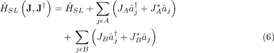
and treat the hopping term and the additional external source terms as perturbations.
It is quite straightforward to get the grand-canonical free energy of the system as power series of both the hopping parameter t and the external source  via Taylor expansion. Since the unperturbed ground states are either Mott phases or CDW states, J and
  can only appear in pair, after re-grouping the terms in the free energy with respect to J and
  , the free energy reads
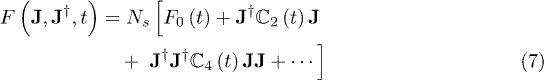
with the expansion coefficient tensor 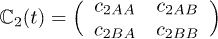 being
being 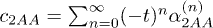 ,
,  ,
,  , Ns is the total number of the lattice sites.
Due to the nature of the superlattice structure of the system, the superfluid order parameter takes the form of the vector  whose components are defined as
  which can be calculated from the free energy by [34]
  .
.
A Legendre transformation of the free energy  leads to an effective potential
  which is expressed in terms of
  as
as

this takes exactly the form of the Landau  theory. According to the Landau theory,
  determines the phase boundaries between the uncompressed Mott or CDW states and superfluid phases. It is not difficult to find out that
  , hence, the critical value of t can be found by looking for the radius of convergence of the determinant of
  :
:

There is no odd order term of t because  has only even terms, while
  has only odd terms. The convergence radius may be found via the so-called d'Alembert's ratio test, and the n-th–order approximation of the phase boundary reads

Process chain calculation and the quantum phase diagram
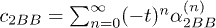
From the above discussion, we see that in order to find the critical value of t to determine the phase boundaries, the coefficients of  have to be calculated out, this can only be achieved perturbatively. Since the unperturbed state is a Mott state or a CDW state, every nonzero contribution to
  includes exactly one creation operator at site i (associated with Ji) and one annihilation operator at site j (associated with
  ) as well as n nearest-neighbor hopping processes (associated with t) connecting site i and j.
Actually, when calculating many-body problems, a perturbation theory as the Rayleigh-Schrödinger perturbation expansion [35] may be applied, with the help of Kato's formulation of perturbation series [32] and process chain technique [31], results with very high-order correction may in principle be reached. Let us denote the ground state of  by
by  . In general, when
  is subject to some perturbation V, the eigenenergy of the total Hamiltonian
  can be perturbatively expressed as
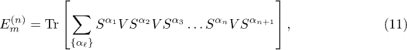
  with the n-th–order correction given by the trace [32]
the operators  connecting each perturbation terms V read
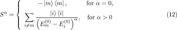
with  and
and  the unperturbed energies of the
  's eigenstates
  and
and  . Since the eigenstates of
  form an orthonormal basis, it is easy to prove that
  , for,
  , and
, and 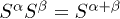 for
for  . It should be emphasized that all possible sequences of
  with constraint
  must be taken into account in the calculation [31,32].
Each Kato term  in eq. (11) represents a sum of processes going from the ground state
  over series of different intermediate states
  , caused by the perturbation V, then back to
  , i.e. the Kato terms are sums of the so-called process chains [25,31].
In our case, the perturbation terms are hopping terms and external source terms, and the unperturbed ground state  stands for the Mott or CDW state. All these process chains can be abstractly represented by diagrams [31], due to the linked-cluster theorem [35], only connected diagrams contribute. As an example, we show in fig. 1 topologically different diagrams for sixth-order perturbations consisting of exactly one source in (denoted by a dot
  in the diagram), one source out (denoted by
  ) and four hoppings between nearest-neighbor sites (denoted by arrows).
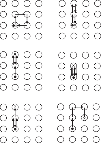
Fig. 1: Sketch diagrams for topologically different processes of sixth-order perturbation terms, consisting of exactly one creation  , one annihilation
  and four nearest-neighboring hoppings (arrows in diagrams).
Download figure:
Standard imageBy applying the above sketch process chain method to the calculation of all  needed, together with eq. (10), the phase boundaries between the Mott (or CDW) state and the superfluid phase can then be calculated. The quantum phase boundaries of the ultra-cold Bose system in a square superlattice with
  are shown in fig. 2 up to the 8th order. The comparison to Monte Carlo numerical results [30] shows that the relative deviation of our 8th-order process chain results from the Monte Carlo results is less than
  .
.
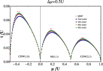
Fig. 2: (Color online) The quantum phase diagram of an ultra-cold Bose system in a square superlattice with  . The quantum Monte Carlo numerical simulation result [30] is also shown.
Download figure:
Standard imageA more accurate result may further be obtained via the linear fit extrapolation method [25,31]. When plotting the logarithm of the coefficients  against the order of n, i.e. the number of tunneling processes in the perturbative calculation, for different ground states (CDW or MI), we find a good linear behavior, as shown in fig. 3. This indicates that, in a good approximation, the ratio between the coefficients of adjacent orders is constant, and would be exact in the case of infinite dimensionality [31]. However, due to the tunneling perturbation, the ratio would change slightly when increasing the order n. As is known, in order to get the exact convergence radius of a power series via d'Alembert's ratio test, the order n should be sent to infinite. Based on the data of order 2, 4, 6, and 8 obtained above, the extrapolation over
  can be carried out, and we can then obtain the critical value of tc for different μ when
  . As shown in fig. 4, our result is nearly identical with the numerical result [30]. By selecting different orders when doing the extrapolation, we find that the relative error of our result is less than 1%.
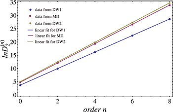
Fig. 3: (Color online) Logarithm of  vs. the order n in different cases, lines are corresponding linear fits.
Download figure:
Standard image
Fig. 4: (Color online) The quantum phase diagram of an ultra-cold Bose system in a square superlattice with  from the extrapolation. The quantum Monte Carlo numerical simulation result [30] is also shown. A good agreement is exhibited.
Download figure:
Standard imageThe TOF pictures
In our previous work [29], with the help of re-summed Green's function method [27,29], we have calculated analytically the TOF pictures of a Bose-Hubbard system in a triangular optical lattice. A generalized Green's function method [36] has also been developed to tackle problems of a Bose-Hubbard system in a bipartite optical lattice. In this section, by utilizing the generalized Green's function method, we will investigate the TOF of the Bose-Hubbard model on a square superlattice.
As is known, the superlattice Bose-Hubbard Hamiltonian in eq. (1) is the single-band approximation of the many-body Hamiltonian ![$H=\int \text{d}\textbf{r}\psi^{\dagger}(\textbf{r})[-\frac{\hbar^2 \nabla^2}{2m}+V(\textbf{r})]\psi(\textbf{r})+\frac g2\int \text{d}\textbf{r}\psi^{\dagger}(\textbf{r})\psi^{\dagger}(\textbf{r})\psi(\textbf{r})\psi(\textbf{r})$](https://content.cld.iop.org/journals/0295-5075/113/1/16004/revision1/epl17631ieqn76.gif) in the tight-binding limit at extremely low temperature [37], the optical lattice potential
in the tight-binding limit at extremely low temperature [37], the optical lattice potential  is [38]
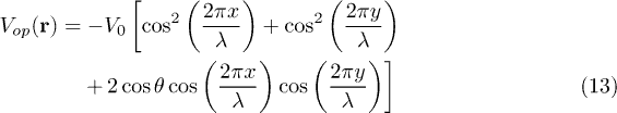
which creates the checkerboard pattern of the square optical superlattice with alternate deep and shallow wells and the relative well depth can be tuned in real time by changing the phase difference  between the counterpropagating laser beams. The lattice constant
  with λ being the wavelength of the laser.
In the harmonic approximation, we expand the optical lattice potential in the vicinity of sublattice A (the locations of deep wells, the sublattice which the site  belongs to) and sublattice B (for instance the site
  ), respectively, and easily get the harmonic-oscillator frequencies
  for deep wells (+ sign) and shallow wells (− sign). Correspondingly, in unit of recoil energy
  , the lowest-band Wannier functions for sublattices A and B read
 ![$w(\textbf{r}-\textbf{r}_{i})|_{i\in A,B}=[\tilde{V}_{0}(1\pm\cos\theta)]^{\frac{1}{4}} (\frac{\pi}{a^{2}})^{\frac{1}{2}} \exp[-\frac{\pi^{2}}{2}\sqrt{\tilde{V}_{0}(1\pm\cos\theta)}\frac{(x-x_{i})^{2}+(y-y_{i})^{2}}{a^{2}}] $](https://content.cld.iop.org/journals/0295-5075/113/1/16004/revision1/epl17631ieqn84.gif) with
with  .
.
When expanding the field operator  in the basis of the orthonormal Wannier function
  ,
, 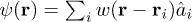 , we find that the hopping parameter t and the on-site interaction U are determined by [37]
  and
and  , respectively. Meanwhile, from the expression of the optical lattice potential in eq. (13), we see that
  .
.
The density distribution function in momentum space [39] reads  which can in turn be expressed in terms of the
 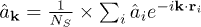 as
as 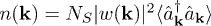 [40], or in other words,
  , where
 ![$G(\tau |0,\textbf{k})\equiv\langle\hat{T}_{\tau}[\hat{a}^{\dagger}(\tau)_\textbf{k}\hat{a}(0)_\textbf{k}]\rangle$](https://content.cld.iop.org/journals/0295-5075/113/1/16004/revision1/epl17631ieqn96.gif) is the Fourier transformation of the one-particle Green's function
is the Fourier transformation of the one-particle Green's function ![$G(\tau', j'|\tau, j) \equiv\langle\hat{T}_{\tau}[\hat{a}^{\dagger}_{j'}(\tau')\hat{a}_j(\tau)]\rangle$](https://content.cld.iop.org/journals/0295-5075/113/1/16004/revision1/epl17631ieqn97.gif) . By treating the hopping term in eq. (1) as perturbation, in the Dirac picture, the Green's function reads
. By treating the hopping term in eq. (1) as perturbation, in the Dirac picture, the Green's function reads ![$G(\tau',j'\mid \tau,j)=\,\frac{\text{Tr}\{{{e^{-\beta \hat{H}_{0}}}\hat{T}_{\tau}[\hat{a}^{\dagger}_{j'}(\tau')\hat{a}_{j}(\tau)\hat{u}(\beta,0)]}\}} {\{\text{Tr}{e^{-\beta \hat{H}_{0}}}\hat{u}(\beta,0)\}}$](https://content.cld.iop.org/journals/0295-5075/113/1/16004/revision1/epl17631ieqn98.gif) , where
, where  , and
, and ![$\hat{u}(\beta,0)=\hat{T}_{\tau}[\exp(\int^{\beta}_{0}\text{d}\tau\sum_{\langle i,j \rangle} t\hat{a}^{\dagger}_{i}(\tau)\hat{a}_{j}(\tau))]$](https://content.cld.iop.org/journals/0295-5075/113/1/16004/revision1/epl17631ieqn100.gif) is the evolution operator (setting
is the evolution operator (setting  ) [41]. After expanding the evolution operator perturbatively, it is not difficult to see that the expansion of the Green's function consists of terms as
 ![$\frac{1}{n!}\sum_{i_{1},j_{1},\ldots,i_{n},j_{n}}t_{i_{1},j_{1}}\cdots t_{i_{n},j_{n}}\times\int^{\beta}_{0}\text{d}\tau_{1} \cdots \int^{\beta}_{0}\text{d}\tau_{n} \langle\hat{T}_{\tau}[\hat{a}^{\dagger}_{j'}(\tau')\hat{a}_{j}(\tau)\hat{a}^{\dagger}_{i_{1}}(\tau_{1}) \hat{a}_{j_{1}}(\tau_{1})\cdots\hat{a}^{\dagger}_{i_{n}}(\tau_{n})\times\hat{a}_{j_{n}}(\tau_{n})]\rangle_{0}$](https://content.cld.iop.org/journals/0295-5075/113/1/16004/revision1/epl17631ieqn102.gif) with
with  being the average quantity with respect to
  , in other words, n-particle Green's functions
 ![$G_n^{(0)}=\langle\hat{T}_{\tau}[\hat{a}^{\dagger}_{i_{1}}(\tau_{1}) \hat{a}_{j_{1}}(\tau_{1})\cdots\hat{a}^{\dagger}_{i_{n}}(\tau_{n})\hat{a}_{j_{n}}(\tau_{n})]\rangle_{0}$](https://content.cld.iop.org/journals/0295-5075/113/1/16004/revision1/epl17631ieqn105.gif) with respect to
with respect to  need to be calculated out, and this can be achieved by expanding them in terms of cumulants [27–29]
 ![$C^{(0)}_m(\tau'_{1},\ldots,\tau'_{m}|\tau_{1},\ldots\tau_{m}) =\langle \hat{T}_{\tau}[\hat{a}^{\dagger}(\tau'_{1})\times\hat{a}(\tau_{1})\cdots \hat{a}^{\dagger}(\tau'_{m})\hat{a}(\tau_{m})]\rangle_{0}$](https://content.cld.iop.org/journals/0295-5075/113/1/16004/revision1/epl17631ieqn107.gif) . However, since we are dealing with a system on a superlattice, according to the generalized Green's function method [36], the cumulants
. However, since we are dealing with a system on a superlattice, according to the generalized Green's function method [36], the cumulants ![$C^{(0)}_{mA}=\langle \hat{T}_{\tau}[\hat{a}^{\dagger}_A(\tau'_{1})\hat{a}_A(\tau_{1})\cdots \hat{a}_A^{\dagger}(\tau'_{m})\hat{a}_A(\tau_{m})]\rangle_{0}$](https://content.cld.iop.org/journals/0295-5075/113/1/16004/revision1/epl17631ieqn108.gif) on sublattice A and cumulants
on sublattice A and cumulants ![$C^{(0)}_{mB}=\langle \hat{T}_{\tau}[\hat{a}_B^{\dagger}(\tau'_{1})\hat{a}_B(\tau_{1})\cdots \hat{a}_B^{\dagger}(\tau'_{m})\hat{a}_B(\tau_{m})]\rangle_{0}$](https://content.cld.iop.org/journals/0295-5075/113/1/16004/revision1/epl17631ieqn109.gif) on sublattice B are different and have to be treated separately.
on sublattice B are different and have to be treated separately.
In practice, the Green's functions can only be calculated out perturbatively by selecting specific groups of terms in the above cumulant expansion expressions in a proper way. According to the re-summed Green's function method [27,29,36], to the lowest order, only terms consisting of first-order cumulants are picked up. In terms of Matsubara frequency, the lowest-order re-summed one-particle Green's function in momentum space reads  where
where  and
and ![$t(\textbf{k})\!=2t[\cos(k_{x}a)+\cos(k_{y}a)]$](https://content.cld.iop.org/journals/0295-5075/113/1/16004/revision1/epl17631ieqn112.gif) . Since
. Since ![$C^{(0)}_{1}\!(\tau)\!=\langle\, \hat{T}_{\tau}[\hat{a}^{\dagger}(\tau) \hat{a}(0)]\,\rangle_{0}$](https://content.cld.iop.org/journals/0295-5075/113/1/16004/revision1/epl17631ieqn113.gif) , by counting the detailed information of the eigenstates of
, by counting the detailed information of the eigenstates of  , in the zero temperature limit, a complicated yet straightforward calculation leads to
  and
and  together with the expression of the unperturbed ground-state energy EnA,nB in eq. (3), the Green's function
  can then be calculated analytically via
  .
.
However, in order to calculate the one-particle Green's function quantitatively and to plot the corresponding TOF absorption pictures, some basic facts and parameters of possible experiments need to be clarified. We may propose that the superlattice Bose-Hubbard model may be realized in experiment by trapping an ultracold 87Rb Bose gas in a cubic optical lattice created by laser beams with wavelength  , the corresponding s-wave scattering length of 87Rb is estimated to be about
  . The superlattice structure is achieved, according to eq. (13), by tuning the phase difference θ. In order to show the alternate Mott and CDW phases, according to the discussion in the second section, we choose θ properly so that
  . In the experiment, in order to eliminate the influence of the third dimension to reveal the 2D properties of the system, the lattice depth in the third dimension
  would be a reasonable choice [11,42,43].
By taking all the above information into account, we calculate and plot the TOF absorption pictures of the superlattice ultracold Bose system released from the CDW(2,1) state and from the MI(1,1) state for different lattice depths in fig. 5 and fig. 6, respectively, it is clear to see that the phases transit from the superfluid phase to the Mott or CDW phase when increasing the lattice depth.
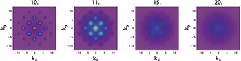
Fig. 5: (Color online) The TOF absorption pictures for various  for an ultracold Bose gas in a square superlattice with its uncompressed state being CDW(2,1). kx and ky in the plots take the unit of
  .
.
Download figure:
Standard imageFrom figs. 5 and 6, we see that the quantum phase transitions of the CDW(2,1) case start to appear with deeper lattice depth when compared with what in the MI(1,1) case, in other words, the quantum critical value of the hopping parameter tc for the CDW(2,1) case is smaller than in the MI(1,1) case, this is in consistence with the quantum phase diagram in figs. 2 and 4. When compared with the TOF pictures of the Bose-Hubbard system in a homogeneous square lattice [1], there are extra peaks at  in the present TOF pictures, this is due to the bipartite superlattice structure, and reflects the inhomogeneity of the superfluid phase.
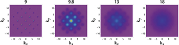
Fig. 6: (Color online) The TOF absorption pictures for various  for an ultracold Bose gas in a square superlattice with its uncompressed state being MI(1,1). kx and ky in the plots take the unit of
  .
.
Download figure:
Standard imageAcknowledgments
The authors gratefully acknowledge Axel Pelster and Tao Wang for their stimulating and fruitful discussions. This Work was supported by National Natural Science Foundation of China under Grant No. 11275119 and by PhD Programs Foundation of Ministry of Education of China under Grant No. 20123108110004.