


Abstract
A common occurrence in everyday human activity is where people join, leave and possibly rejoin clusters of other individuals —whether this be online (e.g. social media communities) or in real space (e.g. popular meeting places such as cafes). In the steady state, the resulting interaction network would appear static over time if the identities of the nodes are ignored. Here we show that even in this static steady-state limit, a non-zero nodal mobility leads to a diverse set of outbreak profiles that is dramatically different from known forms, and yet matches well with recent real-world social outbreaks. We show how this complication of nodal mobility can be renormalized away for a particular class of networks.
Export citation and abstract BibTeX RIS
Introduction
Significant attention among physicists has turned to problems where the dynamics of a meme or virus, plus the network structure on which it is spreading, co-evolve on comparable timescales —whether online [1–3] or in real space [4–13]. Thus a traditional epidemiological description based on mass-action differential equations becomes inadequate. There is a rich variety of works [8–25] that reflect the many possible choices for how a network can evolve dynamically, and hence be modeled to account for detailed real-world mobility patterns [6,7,12,26,27], behavioral effects [28] and environmental factors [5]. In the online world, there are multiple ways in which humans can cluster, including social media communities. Each opens a new pathway for informational contagion (e.g. rumor, idea or plan). Even if the number of individuals actively online in each community is fairly constant, there will be significant churn as people drop in, drop out, and drop back into the conversations over the course of a day, weeks or months [3,22,29–32].
Here we examine the impact of this common dynamical feature of everyday human behavior whereby people join, leave and can rejoin clusters of other individuals  , e.g. by sporadically checking online posts for a particular social media community or re-visiting a particular cafe. The dynamical complication comes from the fact that a returning individual (i.e. node) may find a cluster of individuals (nodes) in which membership has changed very little or a lot, depending on the migration of all the other individuals (nodes). Depending on who they then meet after they enter or re-enter the community, and when, the resulting evolution of any meme or virus at the population level may be very different.
Our model for this co-evolution is purposely very simple (see fig. 1) so that we can write down, and solve numerically, coupled differential equations that mirror the outcome of numerical simulations, as well as enabling some analytical analysis. Yet our simple setup turns out to generate highly anomalous infection profiles which capture the diversity of those observed in recent periods of civil unrest that were fueled by social media (fig. 4). While we do not pretend that our model provides a unique explanation of these real-world phenomena, it serves the purpose of providing a more unified view of such collective social activity. Specifically, our analysis shows that even though a network may appear static on average, an underlying nodal mobility can generate highly nonlinear behavior in an outbreak's severity (i.e. peak infection value H), time-to-peak (i.e. time Tm from beginning of outbreak to its peak), duration T, and area A under the profile I(t). We also provide a novel renormalization scheme that can significantly reduce the complexity of this class of dynamical network problem.
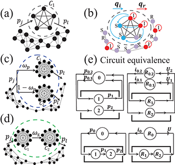
Fig. 1: (Color online) Our simplified model representation of nodal mobility: (a) For a single, internally fully connected cluster C1 embedded in a network. Remaining links are sparse and/or weak (indicated schematically by dashed lines). Probability that a node from outside (or inside) C1 joins (or leaves) the cluster on a given timestep is pj (or pl). (b) For C1 in presence of SIR (Susceptible-Infected-Recovered) process. See text for details. Panels (c) and (d) show the two-cluster case  in parallel and series geometries. (e) Equivalent circuits for M = 2 clusters in parallel (top) and series (bottom).
Download figure:
Standard imageNetwork model
We assume here for simplicity that the M network clusters are internally fully connected (fig. 1(a)) and that for M > 1 the different clusters are interconnected in simple ways, e.g. parallel (fig. 1(c)) and series (fig. 1(d)) by means of sparse links. Given any particular network architecture containing clusters in parallel, series or a combination, our goal is to better understand the impact of allowing nodes to migrate into, out of, and between these clusters such that the overall network appears static on average and yet the identity of the nodes within the clusters can change over time. Consider first a network of N total nodes in which there is a single cluster C1 (fig. 1(a)). At any given timestep, a node from anywhere outside C1 has a probability pj to join C1, while a node inside C1 has a probability pl to leave C1. The number of nodes  in C1 follows
  . For the steady-state situation where
  , the mean cluster size is constant and so the network appears structurally static on average, ignoring individual nodal identity. This mean size
  and the sum of the mean number of nodes joining and leaving is
  . Hence
  characterizes the mean size of C1 and
  characterizes the nodal mobility through C1. At any timestep, an infected agent within C1 transmits a meme or virus to any susceptible within C1 with probability qi (fig. 1(b)). Since C1 is the only fully connected cluster, we will assume that transmission from infected nodes outside C1 is negligible by comparison. Since recovery is individual based, infected nodes inside and outside C1 have probability qr to become immune (for SIR) or susceptible again (for SIS). The infection rate
  is the usual ratio of the infection probability to the recovery probability. Since the S→I process only occurs inside the cluster, we use S(t), I(t), R(t) for the number of susceptible, infected, and recovered nodes in the whole system, and
  ,
,  , and
, and  for the corresponding numbers in the cluster. The six equations that describe the dynamics of an SIR process in this single dynamical cluster situation, are
For an SIS process, there is no immunity for recovered nodes. Hence there are only four dynamical equations:
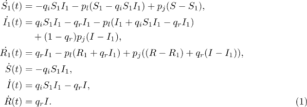
In the simulations, all nodes are initially susceptible and we allow the system to run until the cluster size reaches its steady-state size  . We then randomly pick a node in C1 and make it infected. In every subsequent timestep, all the nodes first carry out the SIR (or SIS) process followed by the joining or leaving of C1. We choose N = 1000. Figure 2(a) shows the trajectory of S and I values in the M = 1 cluster model with SIR, in
  space. The trajectory starts from the lower right-hand corner, as initially we have
  and
and  . The results are in sharp contrast with the standard SIR model in a well-mixed population in which once the infection rate λ and initial number of infecteds I(0) are given, the trajectory is fixed [33]. For the standard SIR in a well-mixed population, if λ and I(0) are given, then there will only be one trajectory in the
  space. The number of recovered nodes R at the end of the outbreak reflects the extent of the infection. We stress that this is real oscillatory behavior, not simply fluctuations. These oscillations (or more generally, resurgent behavior) also appear in results obtained from integrating the set of equations (eq. (1)), although the resulting curve is smoother as an average over many runs is implicitly implied by the equations. In particular, the resurgence arises from the occasional supply of susceptible and infected when nodes join the cluster. For systems larger than 20000 nodes, the oscillations become negligible —however, systems of intermediate size will indeed experience such infection revivals and we stress that such revivals are not caused by simple stochastic fluctuations. The inset in fig. 2(a) illustrates three example profiles. The bottom inset is remarkably similar to the profile obtained for the revaluation of the Chinese Yuan currency reported in ref. [34]. This same rumor circulated twice in the space of a few months, producing an almost identical profile which strengthens the notion that such a profile is not a one-off stochastic aberration. The fact that there was no public announcement or global news to trigger this activity, strengthens the notion that it was caused by spreading through contagion via a mechanism akin to our model.

Fig. 2: (Color online) (a) Trajectories of evolution of the system in the  space for three different sets of parameters. The rough and smooth curves are obtained by numerical simulations and integrating the set of equations, respectively. The parameters are:
  ,
,  , and
, and  (red curves);
  ,
,  , and
, and  (green curves);
  ,
,  , and
, and  (blue curves). The insets show the time dependent of I(t) for each of the cases. (b) SIS (Susceptible-Infected-Susceptible) for one-cluster version. Vertical scale is
  , the normalized fraction of infected nodes in the long-time limit, as a function of
  .
.  ,
,  ,
,  .
.  for simplicity. The inset shows
  as a function of
  . Lines are from integrating the coupled differential equations, symbols are simulation results. (c) Nonlinearity of SIR outbreak severity (I(t) peak height H divided by the constant N which is total number of network nodes) as a function of nodal mobility
  and qi, for different values of the ratio
  for one-cluster version (fig. 1(a)).
Download figure:
Standard imageStrong nonlinear dependences on nodal mobility are also found in the SIS version of the model as shown in fig. 2(b). The panels show the normalized fraction of infected nodes in the long time-limit as a function of  (main) and
  (inset). Similarly to the SIR case, very good agreement is found between the dynamical eq. (2) and the simulations. However, the distinctive component of the SIS case is the non-zero number of infected nodes in the long time-limit, i.e. an SIS epidemic stabilizes over time to a finite value. We find that the effect of nodal mobility and cluster size on the steady state of the infection is highly nonlinear.
While it is known that models with heterogeneity in connectivity or nodal type can produce anomalous infection characteristics as compared to the usual well-mixed SIR model, our model shows this can arise in a network that appears static on average and in which the time-averaged properties of each node are the same, i.e. anomalous infection profiles arise even though each node spends the same average time in cluster C1 and has the same average number of links over time. Figure 2(c) examines the effect of the nodal mobility and infection rate on the outbreak's severity. We find that for small infection rate  , there is a monotonic nonlinear decrease of the outbreak severity with increasing nodal mobility
  . This might be expected since spending less time in the cluster exposes an individual (i.e. mobile node) to less risk of infection. However, one could imagine a competing mechanism whereby increased mobility helps refuel the number of infected in a cluster. As λ increases, the interplay of these two yields a critical value of
  . A maximal severity now emerges at finite
  obeying the approximate relationship
  . For a given infection probability qi, the critical value of
  separates a low-
 phase in which increasing nodal mobility yields a decrease in outbreak severity, and a high-
 phase in which increasing
  yields an increase in severity. For
  , the second mechanism dominates and there is a monotonic nonlinear increase in severity as
  increases for all qi. Additional details of the infection profiles include the observation that area A, duration T and time-to-peak Tm tend to be maximal for smaller values of qi, reflecting the slower spreading and hence longer duration. Moreover, as λ increases, the duration, time-to-peak and area become independent of mobility, because the well-mixed limit is approaching and the existence of clusters becomes unimportant.
Two-cluster version and social outbreaks
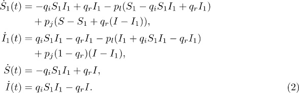
Clusters in parallel (fig. 1(c)) or series (fig. 1(d)) mimic individuals who access one type of space such as a Facebook community, either at the same time as they check another (parallel case) or before they check another (series case). Figure 3 illustrates the rich infection profile behavior I(t) that emerges for parallel (left column) and series (right column) clusters with person-to-person contagion. For the parallel case, we make the simple choice that an agent joins clusters C1 or C2 with probabilities  and
and  , respectively. Hence in the steady state,
  , for
, for  , with
  , and
, and  . The M = 1 case is recovered as
  or
or  . Figures 3(b) and (c) show that the infection peak height H decreases significantly as
  , while fig. 3(a) shows a local maximum at
  . These behaviors are favored by the average size of each cluster becoming similar as
  .
.

Fig. 3: (Color online) Infection profile I(t) vs. time (vertical axis) for different M = 2 cluster geometries and model probabilities (horizontal axis). (a)–(c) Clusters in parallel (fig. 1(c)). (d)–(f) Clusters in series (fig. 1(d)). Profiles calculated by numerical integration of differential equations (see SM) for three parameter sets:  ,
,  ,
,  ((a), (d));
  ,
,  ,
,  ((b), (e));
  ,
,  ,
,  ((c), (f)).
Download figure:
Standard imageFor the series case, we make the simple choice that an agent in C1 joins cluster C2 with probability  and so on for M > 2. An agent in the final cluster CM leaves it with probability pl. Hence in the steady state for M = 2, the differential equations for the population in each cluster become:
In the long-time limit, the mean number of nodes in C1 and C2, respectively, can be written in terms of the mean size parameter for the single cluster case,  :
:
For  ,
,  , where
  , while
  . By contrast for
  ,
,  while for C2 we recover the equilibrium population for the single cluster version (fig. 1(a)). The asymmetry in figs. 3(d)–(f) for M = 2 clusters in series is strikingly different from the symmetry shown for the parallel case (figs. 3(a)–(c)). This asymmetry has its roots in the breaking of symmetry in time (i.e. a node passes through C1 before C2). In addition, figs. 3(d)–(f) also show that as
  grows, the infection profile gradually becomes less dependent on it. Indeed, when
  grows much larger than the probability of leaving C2, pl, the profiles become identical to the M = 1 case and
  becomes irrelevant. Thus, the infection profiles for the series case experience their largest variation for small
  , with infection peaks that are significantly higher than for larger
  . This is because at low
  , C1 has many nodes on average and these nodes are more likely to get infected and hence infect others. As
  grows much greater than pl, the size of C2 approaches the M = 1 case while the size of C1 falls to zero. As a result, the infection profiles become identical to the M = 1 case.
Next, we compare the variability and saturation effect in the time-to-peak Tm for one- and two-cluster versions. So far we have looked at epidemics that require at least one infected node within the cluster so that they could arise. We call this a person-to-person mechanism. An alternative case that we consider now is a broadcast mechanism, in which the nodes residing on one of the clusters experience a constant probability of getting infected regardless of the number of infected nodes present in the cluster. For the one cluster version, we will use the standard person-to-person infection mechanism. For the two-cluster version, we will choose the first cluster to have person-to-person infection while the second is broadcast, e.g. the first cluster mimics individuals in an online chatroom community while the second mimics individuals listening to the same radio broadcast. Two-cluster combinations, with this choice of infection mechanism, can produce a larger ratio  when compared with the one-cluster version, as illustrated in fig. 4(a). Specifically
  as observed in the empirical data (fig. 4(b)). Interestingly, the two-cluster series combination in fig. 4(a) yields a near constant ratio
  for small values of mobility
  but Tm saturates as T increases for larger
  – by contrast, the one-cluster version shows the opposite trend. This calculation for the parallel model reveals an analogous trend to the one-cluster version with minimal variations, hence it is not shown in the figure.
The on-street civil unrest data (colored dots) in fig. 4(b) come from a unique multi-year, national research project involving exhaustive protest event analysis by subject matter experts (SMEs) across Latin America (see refs. [35,36]). The start and end of each outbreak is identified using the analysis of ref. [37] and cross-checked manually. Figure 4(b) shows how the time-to-peak  and duration
  of civil unrest outbreaks (color dots) relates to those generated from our model. The single cluster model captures outbreaks where
  (see middle and bottom simulation curve in fig. 4(b)) while M = 2 clusters in series extends the model's descriptive range to
  in agreement with the data (fig. 4(b) main panel). This is consistent with individuals in the real world, as in the model, sporadically joining and leaving online and/or offline communities in which the idea of creating on-street protests is beginning to circulate. Hence the model's outbreak profile and the actual on-street protest outbreak profile should look similar, as they do.
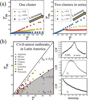
Fig. 4: (Color online) (a) Nonlinear relationship between outbreak time-to-peak Tm and duration T as λ is varied. Left: one-cluster version with person-to-person infection mechanism. Right: two-cluster series version where C1 and C2 experience person-to-person and broadcast infection mechanism, respectively (see text). Values are averages over simulation runs and we have used  for the series case. (b) Time-to-peak
  and duration
  average values for empirical civil unrest outbreaks (colored dots) [36]. Solid lines show
  and
and  as guide. Unlike the one-cluster model, two-cluster versions include the range
  where many datapoints lie. Right: middle and bottom: example infection profile for one-cluster version; top: two-cluster version in series.
Download figure:
Standard imageRenormalization and circuit equivalence
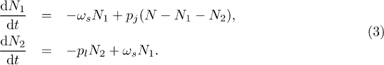
The general case of M > 2 clusters allows for an interesting connection between the nodal migration dynamics and electric circuits (fig. 1(e)) and a novel renormalization. We use k as the cluster label, pk as the probability to leave cluster k, and nk as the number of nodes in cluster k. We can associate an effective resistance  , potential difference
  and current
  . This equivalence allows us to then generalize our model to M clusters connected either in series or in parallel and hence quantify its dynamics. We have established this mapping exactly for M > 2 clusters that are either all in series or in parallel. As an illustration in the steady state, the number of nodes in each of M clusters connected either in series or in parallel is as follows:
where k = 0 represents the nodes outside the fully connected set of clusters; N is the total number of nodes; p0,j is the probability of moving from cluster 0 to cluster j and superscripts s and p denote series and parallel cases, respectively. For the series case, we can then regard the first  clusters as a renormalized super-cluster 1' and replace the last cluster by cluster 2' with the following steady-state populations:
where  is the effective probability of nodes from cluster 1' migrating to cluster 2'.
  is the migration probability from cluster k to adjacent node k + 1 in series. Similarly, for the parallel case we can implement an analogous renormalization so that the size of the super-cluster 1' and cluster 2' can be written as
where  is the effective probability of joining the super-cluster while here the product
  is the probability to join cluster i. With this renormalization, effective two-cluster differential equations can then be written down and solved for the general M case.
Conclusions
In summary we have shown that nodal migration through a network generates highly complex outbreak profiles, even though the network may appear static on average. The introduction of this dynamical feature yields infection patterns that mimic empirical data, specifically outbreaks of civil unrest. These patterns lie beyond the scope of traditional epidemiological models. In addition, we find significant differences in the infection profiles for broadcast transmission within a cluster as compared to person-to-person. This suggests distinct containment policies should be explored for outbreaks whose root cause is infected transient individuals (e.g. hospital patients or airline travelers) as opposed to infected transient places (e.g. the hospital or airport itself). We have also indicated how the complex throughput of nodes can be renormalized exactly for a particular class of dynamical network.
Acknowledgments
We are grateful to Chaoming Song and Stefan Wuchty for detailed discussions. NFJ gratefully acknowledges support from National Science Foundation (NSF) grant CNS1500250 and Air Force (AFOSR) grant 16RT0367.