


Abstract
It is now well established that external stresses alter the behaviour of cells, where such alterations can be as profound as changes in gene expression. A type of stresses of particular interest are those due to alternating-current (AC) electric fields. The effect of AC fields on cells is still not well understood, in particular it is not clear how these fields affect the cell nucleus and other organelles. Here, we propose that one possible mechanism is through the deformation of the membranes. In order to investigate the effect of AC fields on the morphological changes of the cell organelles, we modelled the cell as two concentric bilayer membranes. This model allows us to obtain the deformations induced by the AC field by balancing the elastic energy and the work done by the Maxwell stresses. Morphological phase diagrams are obtained as a function of the frequency and the electrical properties of the media and membranes. We demonstrate that the organelle shapes can be changed without modifying the shape of the external cell membrane and that the organelle deformation transitions can be used to measure, for example, the conductivity of the nucleus.
Export citation and abstract BibTeX RIS
Introduction
The effects of electromagnetic fields on human health have been a concern for a long time and remain a subject of debate. The debate has intensified lately due to the widespread use of cell phones and other electric devices that function close to the human body. The radio frequencies of such devices range from 3 kHz to 300 GHz [1]. Cells in the human body exposed to these fields will respond in a manner still unknown. In vitro experiments have shown that cells can be oriented and deformed with AC fields [2]. The phenomena of dielectrophoresis and electrorotation are also well known [3]. Even more interesting, it is known that the electrical properties of a cell change when pathological conditions develop [4–6]. If electric fields deform the cell, then it is expected that all organelles are affected. Organelles are often enclosed by a lipid bilayer and the nucleus is even surrounded by a double bilayer. The nucleus is the control center of the cell, that is why we focus our attention on this organelle. Indeed, it has been shown that changes in cell shape results in modifications of nuclear shape and functions [7–9]. Cell shape changes in endothelial cells have been associated with nuclear shape remodeling [10] resulting in regulation of gene expression [11,12]. These changes in the nucleus would depend on its mechanical properties, being perhaps more pronounced on cells with softer nuclei. As it turns out, changes in the mechanical properties of cancer cells have been studied in recent years [13], and it has been shown that cancer cells are more compliant than healthy cells [14,15]. However, it has also been shown that infected and cancer cells can be stiffer [16,17] than healthy cells and in some cases, the increase in stiffness can result in apoptosis [18,19]. The effects of AC electric fields on cells are diverse, depending on the target cell and exposure conditions, which makes comparing the experimental results difficults due to the different parameters used (frequency and strength of the electric field, external conditions, different electrode types, and arrangements, etc.). Nevertheless, there is an agreement on the effects on cells at low intensity, intermediate frequency, electric fields. For example, intermediate electric field frequencies inhibit cancerous growth in vitro [20,21] and induce cell cycle arrest and abnormal mitosis by causing the malformation of microtubules that results in cell destruction [22]. In order to study the deformation of cells by AC electric fields we use an oversimplified model of the cell, hereinafter referred to as cell-like system (CLS). Our CLS consists of two concentric spheres, see fig. 1. Each sphere, which is treated as a lossy dielectric, is a bilayer membrane representing the plasma membrane of the cell (external sphere) and the nuclear membrane (internal sphere). Experimentally, CLS are vesicles with sizes of  , known as giant unilamellar vesicles (GUVs), that provide a very simple model for the interaction of electric fields with the cell membrane [23]. When vesicles are exposed to electric fields an electric potential is generated through the membrane and an effective electric tension is induced. The bending and stretching of the membrane by such tension has been studied theoretically [24–26] and experimentally [27]. The main results of these studies demonstrate that vesicle deformations depend on the mechanical properties of the vesicles, the electrical properties of the surrounding media, and the lipid membrane.

Fig. 1: Model. Two concentric spherical shells are immersed in a solution of electrical conductivity  and dielectric constant
  . The outer membrane electric properties are
  ,
,  and the inner shell membrane electrical properties are
  ,
,  . The nuclear interior and the intermediate media have values
  ,
,  , and
, and  ,
,  , respectively. The direction of the alternating applied electric field is illustrated with a bold arrow. The thicknesses of the plasma and nucleus membrane are lm and ln, and membrane and nucleus radii are rm and rn, respectively.
Download figure:
Standard imageThe model
In this paper we calculate the deformations and transition shapes of the nucleus and plasma membrane in a CLS model as a function of the frequency of the electric field and the electrical properties of the media and membranes.
The bilayer membranes in our CLS model have thicknesses lm and ln for the membrane and the nucleus, respectively. The deformations of a membrane due to an AC electric field lead to an increase of the bending energy, adopting prolate and oblate shapes. We consider the deformation to be prolate if the polar radius is greater than the equatorial radius of the spheroid, and oblate if the polar radius is smaller than the equatorial radius. In this work, the z-axis is parallel to the polar radius. To describe the change in elastic energy we use the bending energy introduced by Winterhalter and Helfrich [24]

where,  and
and  , si is the deformation amplitude, ki is the membrane bending rigidity of the membranes, and Msp(i) is the spontaneous curvature. The membrane and nuclear radii are defined as
  and
and  , respectively, see fig. 1. The shapes of the deformed membranes are described by
  . Where
  is the unit vector in the r direction and u is the displacement vector, of which the components are:
  and
and  [24], satisfying the requirement of local area conservation. This vector describes the deformation as oblate or prolate. Throughout this work the spontaneous curvature is assumed to be zero. If si > 0 the deformation is prolate, if si < 0 the deformation is oblate, consistent with our agreement on the direction of the field and membrane deformation explained above. The conductivity and dielectric properties of our CLS model are indicated in fig. 1. We assume small membrane deformations and compute the electric fields assuming spherical shapes at all times. In this work, magnetic fields are neglected and the wavelengths used are much smaller than the CLS characteristic size, therefore, we use the quasi-static approximation of the Maxwell equations,
  .
.
In general, the electric field has the form

where  . The Laplace equations for all 5 regions in fig. 1 can be solved to find the electric potentials with the following boundary conditions:

where  , with t and n corresponding to the tangential and the normal components of the electric field and
  . The electric potential has the well known form:
  , so the time-independent electric field can be expressed as:

where the functions  and
and  are given by

the a's and b's constants are obtained by using the boundary conditions (eq. (3)).
The Maxwell stress tensor is calculated in order to compute the force densities over the membranes. The cases of interest are those for stationary deformations induced by time-independent terms, which can be obtained by averaging over a period of  [26]. The force densities are given by

the bracket denotes average and the dot represents the product between a tensor and a vector. The work generated by the force densities over the membranes can be calculated using

where

and  . Integrating over all the membrane surface we obtain for the nucleus and plasma membrane:

where E0 is the amplitude of the external electric field, and  is
is

The electric properties of the media, membranes, and the frequency of the electric field are in the  factors. The total free energy of the membranes that are subjected to an AC electric field are given by

Minimization of the free energy yields the degree of deformation in our CLS, which is

Results
From eq. (12) a morphological diagram of deformations (MDD) can be generated in the conductivity-frequency space. Transitions are identified by inspection of the changes in sign of si. Theoretically, we can manipulate the conductivity of the media, that includes the electrical conductivity of the membranes and the inner medium. By setting  ,
,  and
and  , we reduce our CLS to a single bilayer system. By using experimental values reported in the literature for GUVs deformations [26–28], we obtain the same morphological diagram reported in these publications. The MDD for these conditions is represented by the external membrane of the ellipsoid, see fig. 2. When r5 < r4 < r3, we have two concentric membranes in our system. Both membranes are illustrated in fig. 2, where the inner membrane does no show deformations for x > 1 and only oblate deformation for x < 1. Here
  .
.

Fig. 2: Morphological diagram of deformations for a single vesicle. The shapes of the deformations are represented by the ellipsoids. The external ellipsoid corresponds to the case of one single membrane. When two concentric membranes are present the effects on the inner ellipsoid are illustrated. Oblate deformations are observe for conductivity ratios,  , lower than one. No deformations are observe for conductivity ratios larger than one. Line transitions illustrate: 1) Prolate-to-oblate transition of the external membrane; 2) oblate-to-sphere transition; 3) Prolate-to-Sphere transition; and 4) Transition obtain by varying the conductivity ratio, which depends on the frequency. The positive direction of the z-axis is shown by the arrow and this direction is the relative direction of the electric field. The numerical values for a single membrane are those reported in the literature [26,27]. The numerical values for two membranes are
  ,
,  ,
,  ,
,  ,
,  , and
, and  .
.
Download figure:
Standard imageTo obtain a MDD for parameters in physiological conditions we used values reported for cells [29,30] and are given by:  ,
,  ,
,  ,
,  ,
,  ,
,  ,
,  ,
,  ,
,  ,
,  ,
,  , and
, and  . The membrane deformations will depend on the field frequency and the ratio of the conductivities. We define the external and internal conductivity ratios as
  and
and  , respectively. We start our analysis by taking the experimental values
  , and
, and  , for which
  . Thus, xint > 1, see fig. 3. The MDD shows a similar behavior for the inner membrane but with an oblate-to-prolate transition at nearly
  , see line transition 2 in fig. 3, and an prolate-to-sphere transition at higher frequencies, line transition 3 in the same figure. A new tansition is predicted for the external membrane that depends on both the electric field frequency and xext, line transition 1 same figure. For a CLS model we use the conductivity values of the cytoplasm and inner nucleus reported in the literature [30]. It is observe here that is possible to deform the inner membrane without deform the outer membrane, as seen along the transition line number 1 shown in fig. 3 at high frequencies. Note that if we increase the strength of the conductivities, there is a shift in the frequency transitions as shown in figs. 3 and 4.
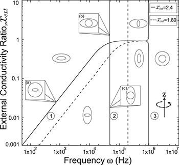
Fig. 3: Morphological diagram of deformations. The ellipsoids are a cartoon representation of the shapes of the nucleus (inner ellipsoid) and plasma membrane (external ellipsoid) of the CLS. The positive direction of the z-axis is shown by the arrow. Solid and dashed lines correspond to the conditions indicated in the upper right box,  ,
,  (solid line) and
  ,
,  (dashed line).
Download figure:
Standard image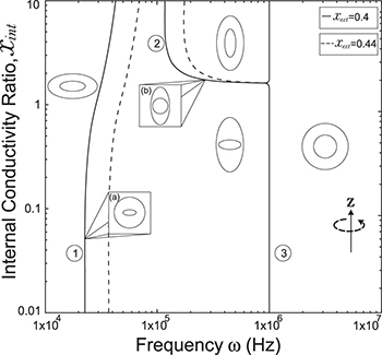
Fig. 4: Morphological diagram for the nucleus conductivity variations. The positive direction of the z-axis is shown by the arrow. The line transition 1 corresponds to the membrane transition and line transition 2 corresponds to the nuclear transition. Solid lines is for  ,
,  and dashed lines for
  ,
,  . In both cases xext < 1.
Download figure:
Standard imageThere is little information about nuclear internal conductivity; therefore, it is interesting to explore the types of deformation when the nuclear conductivity varies. For this, we fix the values of the external and intermediate conductivity,  and
and  , respectively, see fig. 4. For xext < 1, with the transition shapes for the outer membrane are from oblate-to-prolate when the frequency increases and the inner membrane has an oblate-to-prolate transition at larger frequencies, fig. 4. The inner membrane is deformed on the transition line 1 and the external membrane is not perturbed (see inset (a) in fig. 4). On transition line 2, the outer membrane is deformed prolate and the inner membrane has a spherical shape (see inset (b) in fig. 4). In all cases, the deformation of the inner membrane is larger for soft bending rigidity, as expected from eq. (12).
Discussion
The membrane deformations of the CLS explored here can be understood based on the work by Yamamoto et al. [26]. In that work the shape of vesicle deformations were determined by the sign of s, as we did here. The amplitude of the deformation, s, is obtained from the minimization of the free energy, eq. (11), where the positive or negative sign depends on the work done by the second order Maxwell stress tensors. The normal and tangential electric fields embedded in the tensor contribute to the tensile and shear force densities over the internal and external surfaces of the membranes, given by eq. (6), which are the driving forces deforming the membranes. The positive or negative value of these forces are determined by the  's coefficients. Therefore, the sign of s will depennd on these factors: media conductivity, permittivity, the frequency of the electric field. In Yamamotos's work, the conductivity of the membrane was 1010 orders of magnitude smaller than the aqueous solution. The dielectric constant was one order of magnitude smaller than the dielectric constant of the aqueous solution, then
  (with
(with  ). Since
  increase with the frequency ω, the deformations were analyzed in three regions: low-frequency regime (
 where
where  ), intermediate frequency regime,
  , and high-frequency regime,
  and
and  . The low-frequency regime was determined by
  . Using numerical values for a single membrane [26], we obtained approximately
  , below which the stable shape of the vesicle is prolate independently of the frequency of the electric field, in agreement with the experimental results [27]. In comparison, in this work, we used conductivity values that can be three orders of magnitude higher than the conductivities used in [26], while the permitivitty of the membranes is four orders of magnitude larger than the permitivites used in [26]. Using these values we obtained a frequency of 12 Hz as the limit to the low-frequency regime, where deformations are independent of the electric field frequency. The intermediate-frequency regime, where
  and
and  are
are  , which occurs at
  , see fig. 3. Below 12 Hz the prolate deformations are independent of the electric field frequency. This occurs because the electric field is shielded from the internal media or have a weak permeation, and the forces over the external membrane are tangential and a prolate deformation is observed. At frequencies higher than 12 Hz, the high value of the membrane conductivity the displacement currents flow across the membrane, hence a normal component of the electric field appears. The electric field permeates the external membrane and the conductivity of the internal medium reshapes the electric field and the Maxwell stresses. Shear and tensile forces, coming from the Maxwell stresses, deform the membranes. The deformation depend on the conductivity ratios between the inner and external media and the electric field frequency. For xext < 1, the tangential force density acts on the electric charges accumulated at the membrane surfaces. This force will point towards the poles of the membranes. The normal force density at the poles of the membranes point towards the exterior of the vesicle. Therefore, the two resulting forces deform the vesicle in a prolate shape. For xext > 1, there is a change of direction of the forces. The tangential forces point towards the equator and the normal forces at the poles point towards the interior of the vesicles. Both forces deform the vesicle in an oblate shape. The prolate-to-oblate transition comes from the competition between force densities arising from the interaction between accumulated charges at the membranes and the electric fields. At high frequencies, higher than 1 MHz, charge accumulation at the membranes decreases due to the Maxwell-Wagner relaxation frequency. Therefore, the work done by the Maxwell stresses vanishes and we observe spherical shapes as can be seen in figs. 3 and 4. Note that we plot xext vs. ω and in Yamamoto's work is plotted
  vs. ω.
Another important factor in the deformations studied here is the geometry of the system. In the case of a single vesicle, the ratio between the thickness of the membrane and the radius of the vesicle  have an important role in redirecting the electric fields. This implies a competition between geometrical parameters and frequency of the electric field [26]. In this work, the inner vesicle imposes a new constraint on the charge and electric field distribution
  . For low frequencies, the electric fields are redirected tangential over the inner membrane, producing tangential forces pointing to the equator and a normal electric field produces inward forces, deforming the inner membrane in an oblate shape, see figs. 3 and 4. The normal forces over the external and inner membranes counterbalance each other and only tangential forces pointing toward the poles are applied over the external membrane and an oblate shape of the external membrane is observed. By increasing the frequency, the field permeates more and the normal external forces dominate to deform the external membrane in a prolate shape, see fig. 3. The transition line is established by
  , which using the numerical values cited above gives ω ≈ 20 kHz., see fig. 4.
If we plot xint vs. ω, we obtained another morphological diagram, fig. 5. In this case, we varied the internal conductivity of the inner vesicle, we obtained the same transition as the previews morphological diagram for the external vesicle, with a transition line for the inner membrane. This transition depends on the frequency and geometrical factors as explained below.
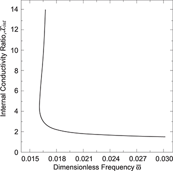
Fig. 5: Bifurcation curve. Using eq. (17) we can reproduce the transition for the inner membrane shown in figs. 3 and 4. The transition occurs either at a constant conductivity ratio xint or at a fixed frequency.
Download figure:
Standard imageThe intensity of the electric field is modified from one medium to another by a factor that depends on the boundary conditions expressed in eq. (3), where the strength of the conductivity media plays an important role. The parameters used in this numerical calculation (taking into account the values reported experimentally), give us  and
and  , then the ratio of the inductances can be expressed as
  and
and  . Taking the limit
  we obtain
  . In this case, the equation of the inner membrane deformation takes a simple form:

where  and the Λ's are constants that depend only on the geometry of the system:
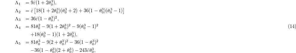

where  and
and  . The numerical values of Λ's constant for
  and
and  are
are
and we can find the bifurcation curve given by

Equation (17) is plotted in fig. 5. This bifurcation curve predicts the behavior of the inner membrane deformation as presented in figs. 3 and 4 (see lines 2). For example, using the numerical value for xint in fig. 3, shows that the frequency transition is constant. While varying xint will yield the different frequencies at which the inner membrane changes shape. This is very important experimentally because it allows us to measure the transitions of the inner membrane without knowing the inner vesicle conductivity. Then, using fig. 5 and eq. (17) we can estimate the internal conductivity of the inner vesicle. It is important to note that the transition occurs only if we take into account the thickness of the inner membrane, because the Λ's depend on the ratio of the inner radii.
To test our theory, experiments could be conducted with double bilayer systems of different sizes by, for example, jet-injection or double emulsion techniques. In cells, experiments could be conducted on detached cells. In this system, our theory could provide a way to measure the conductivity of the nucleoplasm by measuring the shape transition of the nucleus. In this work, we neglected the membrane conductivity that can affect the charge distribution and the nature of the force densities over the surfaces, in order to have a better model, we will have to take into account this factor. However, this is a first step towards more complex models to study the deformation of multi-bilayer membranes or of organelles and cells.
Acknowledgments
We acknowledged financial support from CONACYT through project Nos. 169504 and 440 Fronteras de la Ciencia. We thank A. Ramírez-Saito and M. L. González-González for fruitful discussions. HA-E and KA acknowledge support from NSF (1507730).