


Abstract
The interplay between external field and fluid-mediated interactions in active suspensions leads to patterns of collective motion that are poorly understood. Here, we study the hydrodynamic stability and transport of microswimmers with weak magnetic dipole moments in an external field using a kinetic theory framework. Combining linear stability analysis and non-linear 3D continuum simulations, we show that for sufficiently high activity and moderate magnetic field strengths, a homogeneous polar steady state is unstable and distinct types of splay and bend instabilities for puller and pusher swimmers emerge. The instabilities arise from the amplification of anisotropic hydrodynamic interactions due to the external alignment and lead to a partial depolarisation and a reduction of the average transport speed of the swimmers in the field direction. Interestingly, at higher field strengths the homogeneous polar state becomes stable and a transport efficiency identical to that of active particles without hydrodynamic interactions is restored.
Export citation and abstract BibTeX RIS
Introduction
As a microswimmer propels itself through a fluid, it generates a long-range disturbance. This perturbation propagates through the fluid and influences the motion of other swimmers. Self-propulsion in conjunction with fluid-mediated interactions in active suspensions give rise to a wealth of collective phenomena that are very distinct from those found in passive systems at equilibrium [1–5]. Some examples include hydrodynamic instabilities that lead to spatio-temporal pattern formation [6–8], active turbulence [9–12] and unusual rheological properties [13–16]. Moreover, microswimmers exhibit new motility patterns in response to external stimuli such as chemical signals [12,17,18], light [19,20], gravitational [21–25] and magnetic fields [26–30]. The control and regulation of collective motion of microswimmers via an external field offers a promising route for their exploitation in high-tech applications such as micro-scale cargo transport, targeted drug delivery, and microfluidic devices [31–34].
Presently, a theoretical understanding of collective behaviour and transport of microswimmers in an external field is largely missing. Here, we put forward a kinetic theory for active suspensions that extends the previous kinetic models [6,7] to include the effects of an external field. Our model is applicable to any active suspension driven by an external aligning torque. Examples include magnetotactic bacteria (MTB) carrying an intrinsic weak magnetic moment [35–39] and weakly magnetised artificial swimmers [40–49] in an external magnetic field or bottom-heavy swimmers in a gravitational field [22]. MTB driven by a sufficiently strong magnetic field exhibit particularly intriguing patterns of collective behavior such as band formation [26,27] and pearling instability under flow [28]. Thus, we focus on the dynamics of active magnetic suspensions in a uniform magnetic field.
We investigate the instabilities and transport of dilute suspensions of spherical magnetic swimmers in an external field combining linear stability analysis and 3D numerical simulations. At low magnetic fields, a homogeneous weakly polarised state is stable, akin to an isotropic suspension of spherical swimmers. However, for sufficiently high activity strengths and moderately strong magnetic fields, a homogeneous polar phase becomes unstable for both pushers and pullers. These instabilities significantly reduce the polarisation of the swimmers and lead to a decrease in their mean transport speed. In the unstable regime, we observe a rich phenomenology of pattern formation by varying the magnetic field and activity strengths. Representative examples of pattern development for pushers and pullers are shown in fig. 1. Notably, pushers and pullers exhibit distinct instability patterns that result from the divergence of bend and splay fluctuations [50–52], respectively. The 3D visualisation of the density field in fig. 1(c) and (d) (see also the corresponding supplementary videos pusher.mp4 and puller.mp4) clearly shows that the pushers concentrate in band-like structures perpendicular to the magnetic field that migrate in the field direction, whereas pullers form lane-like patterns parallel to the field. Our results for the pushers are remarkably similar to the observed magnetotactic bands reported for spherical MTB [26,27]. The instability of the polar state induced by an external field shares similarities with the instability of aligned swimmers with nematic or polar interactions [6,7]. However, for an externally induced polar state such an instability disappears by a further increase of the magnetic field strength. To our knowledge such a re-entrant hydrodynamic stability has not been previously reported in active systems and calls for further experimental investigations.
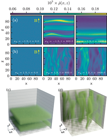
Fig. 1: Snapshots of density projections averaged along the y-axis from 3D non-linear simulations at different time steps for pusher (row (a)) and puller swimmers (row (b)) in the unstable regime with dimensionless active stress  and alignment parameter
  . The colours encode the probability density integrated in the y-direction
  . 3D volumetric rendering of the density field of a pusher (c) and puller (d) at t = 1800 corresponding to the last time step presented in panels (a) and (b), respectively.
Download figure:
Standard imageModel system description
We consider a dilute suspension of N spherical magnetic microswimmers with a hydrodynamic radius a immersed in a fluid of volume V at a number density  . We assume that the self-propulsion is generated by a force-free mechanism of hydrodynamic origin such that the far field flow of a swimmer is well represented by that of a point-force dipole with an effective dipolar strength Seff [7,53–55]. Seff depends on the geometrical parameters of the model swimmer [42,43,45,55], for instance on a and the flagellum length ℓ [55]. Each swimmer carries a weak magnetic dipole moment configuration of an ensemble of the
  along its body axis
  and has a self-propulsion velocity
  . The suspension is exposed to a uniform magnetic field B that exerts an aligning torque on each swimmer. The magnetic moment values of MTB are of the order of
  [36,38,56,57] and their size
  . For dilute suspensions with inter-particle distances
  , their dipole-dipole interactions are small compared to the thermal energy scale and we can neglect their effect. Instead, we focus on the interplay between the hydrodynamic interactions and the aligning torque.
Kinetic theory
For sufficiently low ϱ, the mean-field configuration of an ensemble of the swimmers at a time t can be described by the probability density  of finding a particle with the center-of-mass position x and the unit orientation
  .
.  is normalized such that
  . The time evolution of Ψ is governed by a Smoluchowski-equation of the form

where  denotes the angular gradient operator; Jtr and Jrot are the translational and rotational drift currents.
  , with
  as the Laplace operator on a unit sphere, accounts for the evolution of Ψ resulting from the translational and rotational diffusive currents. Dt and Dr represent the effective long-time translational and rotational diffusion coefficients that can be of thermal or biological origin, e.g., due to tumbling of bacteria.
  describes the translational current stemming from the self-propulsion of a swimmer and its convection in the local flow u,

The rotational current  incorporates contributions from the rotational velocities resulting from the torque generated by the aligning magnetic field and the local flow vorticity
  according to Jeffery's equation [58,59]:

where  is the rotational friction coefficient.
The flow field ![$\mathbf{u}[\Psi]$](https://content.cld.iop.org/journals/0295-5075/125/2/28001/revision1/epl19508ieqn26.gif) in the low Reynolds number limit is captured by the incompressible Stokes equation
in the low Reynolds number limit is captured by the incompressible Stokes equation

in which P denotes the isotropic pressure and η the viscosity of the suspending fluid and  . The flow is determined by the state of the system encoded by Ψ via a mean-field stress profile
 ![$\mathbf{\Sigma}[\Psi]$](https://content.cld.iop.org/journals/0295-5075/125/2/28001/revision1/epl19508ieqn28.gif) . It includes two contributions: an active stress
. It includes two contributions: an active stress  , generated by the self-propulsion of force-free dipolar swimmers [53,54], and an antisymmetric magnetic stress
  , caused by reorientation of swimmers in the magnetic field. The active stress is proportional to the angular expectation value of the nematic order tensor
  [7,60]. The strength of the active stress is given by
  . The sign of
  determines the nature of the swimmers, being a puller
  or a pusher
  . The magnetic stress is given by
  in which
  and
and  [61]. Note that the symmetric part of the stress is zero for spherical particles [61].
To facilitate the analysis of our model, we render the equations dimensionless, using the following characteristic velocity, length, and time scales:  ,
,  (average inter-particle distance) and
  . These scaling choices leave the distribution function unchanged:
  . The corresponding dimensionless model parameters are the magnetic field strength
  , the rotational and translational diffusion coefficients
  and
and  , the active stress amplitude
  and the magnetic stress amplitude
  .
.
Homogeneous steady state solution
Let us first consider a solution of eq. (1) satisfying,  and
and  .
.  is given by

in which  and it is identical to the steady state solutions obtained in [16,28,39]. We call α the alignment parameter as it is equal to the ratio of two characteristic reorientation times;
  .
.  represents the average decorrelation time of the particle from its initial orientation and
  describes the typical time a non-diffusive particle needs to align itself with the magnetic field. Hence, the degree of alignment is determined by the competition between the aligning magnetic torque and the randomizing rotational diffusion. The
  corresponds to a homogeneous polar state with a mean polarization vector
  in which

is known as the Langevin function in the context of paramagnetism. Note that a full alignment is only achieved for  .
.
Linear stability analysis
We investigate the linear stability of the homogeneous polar state by considering a small perturbation of the form  . The equation of motion linearised in
  can be expressed as an eigenvalue problem of the form
  , where
  is a linear differentio-integro-operator (see the Supplementary Material Supplementarymaterial.pdf (SM)). We solve the eigenvalue problem in the basis of spherical harmonics
  numerically by truncating the matrix
  at sufficiently large number of modes such that the convergence of the dominant eigenvalues are ensured. The external field breaks the rotational symmetry. Hence, the stability depends on the direction
  of the perturbation wave vector with respect to the magnetic field direction, which can be characterized by a single angle
  .
.
We first examine the stability of swimmers with moderate values of activity and magnetic field strength leading to  and
and  . The remaining parameters are chosen to be comparable to those of MTB [28] and they are fixed to:
  ,
,  , and
, and  . Figure 2 shows the real part of the eigenvalue with the largest magnitude
  , the so-called maximum growth rate, as a function of
  at various perturbation angles
  . For both puller and pusher swimmers, long-wavelength perturbations dominate the instabilities and destabilize the homogeneous polar state defined by p0. For pushers, fluctuations of the linearised equations in the direction of magnetic field grow fastest whereas for pullers both perturbation directions parallel and perpendicular to B predominate. Thus, we expect pushers and pullers to exhibit distinct instability patterns as confirmed by the non-linear dynamics simulations; see fig. 1.

Fig. 2: The dependence of the largest growth rate  , on the wave number k, for the homogeneous polar steady state given in eq. (5) at several wave angles
  for pushers (top,
  ) and pullers (bottom,
  ). The other dimensionless parameters are fixed to
  ,
,  ,
,  , and
, and  .
.
Download figure:
Standard imageNext, we present the stability phase diagram in which we vary the strengths of both activity  and magnetic field
  . Figure 3 depicts the stability diagram for
  in the
  -plane. The magnetic stress is varied concomitant with α as
  ; the remaining parameters are kept constant at the values given in the caption. With this choice of parameters the diagram should represent an experimentally accessible range. From the linear stability analysis, we determine the border lines that separate the stable from the unstable regions. Note that the steady state
  and its polarization depend on α.
  given by eq. (6) is shown in the right panel of fig. 3. At low values of α where polarization is weak,
  ,
,  remains stable. At moderately strong fields and for
  , the hydrodynamic interactions become amplified as a result of the increased polarization and destabilize the steady state. Strikingly, at stronger magnetic fields the hydrodynamic instabilities can be overcome. At such strong fields, the randomizing effect of the rotational diffusion can be ignored. The magnetic torque
  dominates over the hydrodynamic torque and the steady state becomes stable again. This is a consequence of the fact that for a fixed active stress amplitude the hydrodynamic stress and the resulting torque have an upper bound (perfect polarization), whereas we can increase the external torque by increasing the magnetic field. To examine the validity of these predictions, we study the dynamics of swimmers by non-linear simulations.

Fig. 3: Stability diagram of the steady state given by eq. (5) where we have varied the strengths of active stress  and magnetic field
  assuming a constant volume fraction of
  ,
,  ,
,  , and
, and  . The dimensionless diffusion coefficients are fixed to
  and
and  , based on persistence times of
  at room temperature, and the reduced magnetic stress amplitude is varied as
  accordingly, compatible with experimental findings. The solid lines are determined using linear stability analysis and separate the stable from unstable regions. The circles and stars respectively depict stable and unstable points determined by simulations. The right panel displays the polarization of the steady state as a function of
  given by eq. (6).
Download figure:
Standard imageNon-linear dynamics simulations
We perform non-linear simulations of the kinetic model in three dimensions to study the long-time dynamics and pattern formation resulting from the instabilities. To solve the Smoluchowski equation, eq. (1), with periodic boundary conditions, we use a hybrid stochastic particle based sampling method to obtain  and a spectral method to solve for the flow field
  . For further details see the SM. Probing the stability of
  for different activity and magnetic field strengths by simulations, we find excellent agreement with the predictions of the linear stability analysis, as demonstrated in fig. 3.
  is stable for the parameter points denoted by discs, whereas
  values for which Ψ evolves towards an inhomogeneous time-dependent density profile are depicted by stars. The angular distribution of these unstable states appears to converge towards a steady state, whereas their density fields evolve towards dynamic spatial patterns. In the unstable regime, density and polarization gradients generate a flow with an inhomogeneous vorticity field that is coupled to the swimmers orientations and rotates them away from the
  direction. To quantify these disorienting effects, we measure the time-averaged global polarization defined as
  , where
  (with the simulation time step
  in units of tc) is about an order of magnitude larger than the reorientation time
  . The braces
  define the expectation value. t0 marks a relaxation time after which
  is nearly time-independent despite exhibiting non-stationary patterns (see fig. 3 in the SM). Choosing
  allowed us to obtain sufficient statistics. We find that
  and
and  is independent of the system size for
  (see SM). Figures 4(c) and (d) present the
  as a function of α for pushers and pullers at different activity strengths
  . For moderate
  and α values falling in the unstable regime, we observe a significant reduction in the polarization compared to
  (eq. (6)), shown by the dashed line. The decrease in the mean polarization is stronger for larger activity strengths. Stronger magnetic fields drive the system back into the stable regime and
  agrees with
  in those regions.
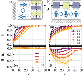
Fig. 4: (a) and (b): idealized streamlines of bend and splay deformations of the polarization field  occurring for pushers and pullers, respectively. The signed squares describe regions with positive and negative divergence of
  and the arrowed circles show the vorticity direction. The blue arrows sketch the local flow profile generated due to the instabilities. (c), (d): the time-averaged polarization magnitude
  vs.
vs.  at different activity strengths
  for pushers and pullers. The dashed line shows the polarization of the steady state given in eq. (6). (e), (f): the time-averaged convection transport speed in the magnetic field direction vs. α at different
  for pushers and pullers. The box size in all simulations is
  . In panels (c) to (e) the confidence intervals are comparable to the symbol size.
Download figure:
Standard imageThe mean polarization governs the mean transport speed  in the direction of magnetic field that additionally includes a contribution from the convective flow component along
  :
:

For an efficient transport in the direction of the magnetic field, a high polarization of swimmers parallel to B is desirable that can be achieved by increasing the field strength. To evaluate the contribution of  to the transport, we calculate the space and time-averaged flow velocity as
  .
.
Figures 4(e) and (f) show  vs.
vs.  for pushers and pullers at different values of
  that is almost independent of box size for
  (see SM). The mean flow velocity created by pushers has a vanishing component along
  . Hence, their transport speed is determined by the mean polarization whereas for the pullers the contribution of convective flow to the transport is significant. This dissimilarity originates from distinct nature of instabilities that prevail the pushers and pullers and distort their polarization field
  , in which
  . For pushers, bending deformations in their polarization field produce alternating shear flow layers perpendicular to
  as schematically drawn in fig. 4(a). Because of imbalance of the magnetic and the flow-induced torques, the bending fluctuations are further amplified and decrease the mean polarization. These distortions also increase the density where
  . As a result, pushers form dense layers perpendicular to
  that migrate parallel to
  , see fig. 1. Similarly for pullers, splay deformations generate alternating pillar-like flow regions along
  as shown in fig. 4(b). Denser regions of pullers where
  coincide with regions carrying a flow anti-parallel to
  . They result in a net convection anti-parallel the magnetic field (fig. 4(f)) and reduce the mean transport speed.
Conclusions
The mean polarization of magnetic swimmers increases continuously with the field at a pace that depends on their activity strength. For  , a weakly polar state is always stable. At moderate fields, for sufficiently strong activities where
  , pushers and pullers exhibit distinct bend and splay instability patterns and propose a pragmatic approach for distinguishing them in experiments. These instabilities highlight the significance of hydrodynamic interactions that hinder the directed transport of swimmers. The reduced transport speed results from the coupling of density and flow field to the distortions of the polarization field. Interestingly, at field strengths beyond an activity-dependent value (
 for
for  and
and  for
for  ) a homogeneous polar state becomes stable. We defer a classification of patterns as a function of activity and magnetic field strengths to a future work.
Finally, we note that our results are valid in the limit of negligible magnetic interactions that are of relevance to dilute suspensions of swimmers with weak magnetic dipole moments such as magnetotactic bacteria. For synthetic magnetic microswimmers with larger magnetic dipole moments or dense suspensions, the magnetic dipolar interactions alone can lead to clustering instabilities [62] and the interplay between long-range magnetic and hydrodynamic interactions on development of instabilities deserves to be explored. Moreover, clarifying the role of swimmer-swimmer correlations [63], and near-field hydrodynamic interactions in more concentrated suspensions merits further investigations.
Acknowledgments
We thank Eric Clément, M. Cristina Marchetti and Friederike Schmid for fruitful discussions and Tapan Adhyapak for a critical reading of the manuscript. We acknowledge the financial support from the German Research Foundation (http://www.dfg.de) within SFB TRR 146 (https://trr146.de). The simulations were performed using the MOGON II computing cluster. This research was supported in part by the National Science Foundation under Grant No. NSF PHY17-48958.