Abstract
Inferring causal relations from empirical data is a central task in any scientific inquiry. To that aim, a mathematical theory of causality has been developed, not only stating under which conditions such inference becomes possible but also offering a formal framework to reason about cause and effect within quantum theory. This perspective article provides an overview of the latest results in the growing field of quantum causality, with a special focus on experimental implementations and concepts that only recently have entered in the quantum information dictionary. Ideas like bilocality, instrumental variables and interventions will be discussed from both a fundamental and an experimental perspective.
Export citation and abstract BibTeX RIS
Understanding cause and effect relations is at the center of any scientific endeavor. It was only in the mid-nineties that a mathematical theory of causality has emerged [1,2] with applications ranging from economics [3–5] to clinical trials [6] and genetics [7,8] to social studies [9], also attracting increasing attention in statistics, machine learning and artificial intelligence [10]. Causality theory allows us to establish a formal connection between empirical data and cause and effect relations. Clearly, however, as it has been long realized, correlation does not necessarily imply causation, and this is the reason why statisticians have historically shied away from causality concepts [2].
The causality framework has been shown to provide a novel perspective in the foundations of quantum physics and quantum information science where three main trends can be observed. First, the language of causal structures provides a natural and intuitive playground to understand and generalize Bell's theorem [11,12]. Causal notions are implicit in virtually any research regarding Bell non-locality, however, it was not until recently that basic causality concepts like common causes, causal influence, interventions and fine-tuning started to appear in the quantum foundations dictionary [13–25]. A second trend is the generalization of the concept of causality itself to the quantum realm [26–36]. Since Bell's theorem we know that our classical notion of cause and effect is incompatible with quantum predictions and that has motivated the search for quantum causality and quantum causal modeling. Finally, a third venue that will only be briefly mentioned in this perspective, has been the idea of indefinite causal structures [30,33,37–43]. At the core of quantum mechanics is the idea of quantum superposition that when applied to causality allows for situations where, as opposed to a classical world, one event is not definitively the cause/effect of the other, the two possibilities happening coherently and (to some extent) at the same time.
In this perspective article we will address, with an experimental insight, some of the most recent developments in quantum causality. With this aim we will discuss central and fundamental concepts in this field.
From causal structures to quantum non-locality
In a typical Bell-like experiment [11,12] two (or more) distant parties perform local measurements on their shares of a joint physical system. By invoking special relativity we have the guarantee that none of the parties can influence the statistics observed by the others. In turn, in a teleportation protocol [44] we have a time-like separation situation where measurements are performed in one laboratory and conditioned on those initial results further actions are implemented on a second distant laboratory. These two paradigmatic situations show that implicit in any quantum information protocol there is an underlying network of potential causes and effects, that is, a causal structure governing the relevant processes and variables.
An intuitive way to define and visualize causal structures is via directed acyclic graphs (DAGs) [2,45]. Each node in the graph denotes a random variable of relevance and the directed edges (arrows) encode their causal relationships. Mathematically, they provide a compact representation of joint probability distributions. Considering a DAG of N nodes  and that Pa(Xi) denotes the graph-theoretical parents of the i-th variable, the so-called Markov condition [45] implies that the joint distribution should factorize as1

The Markov condition (alternatively the DAG) encodes causal relationships via the conditional independences implied by it. To illustrate its central concepts, we analyze next the paradigmatic causal structure in Bell's theorem [12].
In the paradigmatic Bell scenario, depicted in fig. 1(a), two distant parties (Alice and Bob) upon receiving their parts of a joint system choose some measurement to perform (labeled by X and Y), thus obtaining some measurement outcome (respectively, labeled A and B). The source of states and any other relevant physical process that might affect the measurement outcomes (like local noise terms) are represented by the variable Λ. By assumption, the variable Λ is not empirically accessible and thus represents a hidden (or latent) variable. That is, in a Bell experiment we have access to the statistical data represented by the probability distribution p(a, b, x, y) and since the measurements choices are typically under control, it is customary to work instead with the conditional distribution  . Following the Markov prescription (1) for the Bell DAG, this probability can be decomposed as

defining the local hidden variable (LHV) model [11] where two causal assumptions have been employed. First, the locality assumption represented graphically by the absence of direct arrows between Alice and Bob variables and mathematically represented as  (similarly for Bob). Second, the measurement independence ("free-will") assumption, graphically represented by the absence of arrows between Λ and X and Y and thus implying that
  .
.
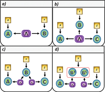
Fig. 1: Causal structures. In DAGs shown here, there are three different kinds of nodes: hidden variables (purple box), measurement settings (yellow boxes) and measurement outcomes (green circles). (a) Paradigmatic bipartite Bell causal structure representing a local hidden variable (LHV) model. (b) Tripartite LHV model. (c) Tripartite scenario with two independent LHVs, that is, a bilocal hidden variable (BLHV) model. (d) Tripartite BLHV model where the central node B is made of two substations BA and BC, driven by the same measurement choice Y.
Download figure:
Standard imageThe DAG approach can be extended to the multipartite scenario. For instance, in the tripartite case, this causal framework already allows to identify two different situations. In the first, all three parties share a state prepared by a common source (fig. 1(b)) while in the second case we might have two or more independent sources (fig. 1(c)). Considering a unique source, the joint distribution should factorize as

In turn, taking explicitly into account the independence of sources as depicted in fig. 1(c) (more explicitly  , the so-called bilocality assumption [46,47]), we now have

All of these descriptions, however, rely on a classical concept of causality that since Bell's theorem we know to be incompatible with the quantum-mechanical predictions. Take, for instance, the bipartite Bell scenario, the statistics observed in such experiment should arise from Born's rule implying that

where  and
and  describe local measurement operators and ρ represents the density matrix for the joint quantum state produced at the source. Bell's theorem shows that quantum correlations described by (5) can be incompatible with the classical causal description provided by (2). The most common way to witness this incompatibility is via the violation of a Bell inequality. Classical causal models such as the LHV models (2) imply testable constraints on the observed correlations. These are precisely the Bell inequalities that, if violated, provide an unambiguous proof of the incompatibility of the observed correlations with the underlying causal model. As quantum correlations violate Bell inequalities, at least one of the two causal assumptions employed in their derivation, locality and measurement independence, must give way in a quantum-mechanical description. As measurement independence ("free-will") is at the core of any scientific quest, that is the reason why this phenomenon is called quantum non-locality. It does not mean that quantum correlations can be used to communicate instantaneously, it just shows that when we try to describe quantum phenomena with a classical notion of causality we arrive at the conclusion that even if very far apart the quantum particles seem to be communicating, the "spooky action at distance" abhorred by Einstein [48].
Given its fundamental importance [11], the violation of the Bell inequalities has been pursued in different physical systems, culminating in the first loophole-free experiments [49–52]. In spite of their groundbreaking nature, most of these experiments focused on the bipartite case or on its straightforward generalization to the multipartite case (always considering a single source of states). As described next, it was only recently, that conceptually different kinds of non-classical correlations started to be considered experimentally.
Experimental violation of bilocality
From direct comparison it is clear that the bilocal set (4) is contained inside the local set (3). More precisely, the bilocal set is characterized by non-linear polynomial Bell inequalities [53–58]. Interestingly, this implies that there exist correlations that might appear classical but have their non-local nature revealed if the independence of the sources generating the correlations is taken into account. Another relevant feature is the fact that the bilocal causal structure reproduces the underlying pattern of causation in a entanglement swapping experiment [59].
In the simplest possible scenario, akin to the entanglement swapping scenario, where Alice and Charlie perform two dichotomic measurements and Bob performs a single measurement with four possible outcomes, the following inequality holds for bilocal hidden variable models [46,47]:

where 
Exploiting the causal structure depicted in fig. 1(c), two photonic experiments have provided an experimental proof-of-principle for network generalizations of Bell's theorem [41,42]. Both considered two different non-linear crystals pumped by the same laser and three different stations where Alice and Charlie make two possible dichotomic measurements and Bob measures in the Bell basis. The maximum violation of the bilocality inequality has reached  corresponding to a violation by almost 20 sigmas [41]. Furthermore, it has been shown experimentally that correlations compatible with a usual LHV model (3) can indeed violate such inequality, thus proving a new kind of non-local correlation.
Similarly to any Bell test, these first violations of the bilocal causality inequality were subjected to loopholes, in particular the locality and detection efficiency loopholes. Another important issue related to these experiments was the fact that both of them exploited just one laser to pump both crystals. Given the nature of the experiments, this introduces a loophole, similar to the measurement independence loophole in Bell's theorem, if the sources of states cannot be guaranteed to be truly independent. To deal with that, Saunders et al. [42] included a random time-varying phase shifter between the crystals in order to increase the degree of independence between the sources and thus to overpass this problem. Another potential issue is the fact that typically Bell experiments rely on a shared reference frame between the parties. While inoffensive in the usual Bell tests, in the case of bilocality such reference frames could be used to simulate non-local correlations with LHV models [43]. Fortunately, however, as demonstrated experimentally in [43], bilocality violations can also be achieved in the absence of shared reference frames.
Recently the group of Pan [60] closed simultaneously the loopholes of source independence and locality in an entanglement swapping experiment, reporting a violation of  , hence rejecting bilocal hidden variable models. One should keep in mind that like in Bell tests we will never be able to rule out a super-deterministic explanation [61], since it is impossible to guarantee that two separate sources are genuinely independent, as they could have been correlated at the birth of the universe (see, for instance, [62,63]).
The experimental verification of the bilocality violation reported in [41,42] has inspired more related works with different approaches [64–72] in which the extension to more complex networks is the central topic of interest. An interesting question was whether the violation of bilocality can be performed in a device-independent way, since the first experiments assumed that Bob's station perform a complete Bell-state measurement with four possible outcomes, something that is impossible with linear optics [73]. In practice this implies that such realizations had to rely on the precise quantum description of the experiment, that is, they were a device-dependent test of bilocality. Notably, it has been shown that quantum mechanics can exhibit non-bilocal correlations also in cases in which all parties only perform single-qubit operations [58], thus allowing for a device-independent test of bilocality with linear optics implementations. To do so, Bob performs separable measurements and hence it is possible to consider the station of Bob as composed by two sub-stations as depicted in fig. 1(d). This experimental approach has been fully addressed [43] and allowed a violation of bilocality with separable measurements up to  .
.
Instrumental causality
A recent development with fundamental importance in the field of causal inference is the so-called instrumental causal structure. Its relevance stems from the fact that it allows to put bounds on the causal influence of a variable A on a variable B, simply based on observational data and without the need of interventions. It relies on a instrumental variable X that is assumed to influence only A directly and to be independent of the shared correlations between A and B. The instrumental DAG (see fig. 2(a)) implies that any correlation compatible with it should be decomposable as

Considering that all observable variables are binary, it has been shown that all quantum correlations, obtained by Born's rule as

are compatible with a classical causal description [29]. However, considering that the instrumental variable assumes three possible values it was shown that there are quantum violations of the instrumental constraints. Quantum correlations of the form (8) can violate the instrumental inequality [74]

where  up to the limit of
  .
.

Fig. 2: Different scenarios within the instrumental causal structure. (a) The instrumental scenario, where X stands for the instrument, A and B are the variables for which we want to estimate causal influences, and Λ represents any latent factor correlating them. (b) Causal relaxation where direct influences between the instrument X and the variable B are allowed. (c) Representation of an intervention on A, performed under the causal influence of a variable I (yellow triangle) controlled by the experimenter.
Download figure:
Standard imageThe violation of this inequality has been reported for the first time in [74] which, opposite to the usual Bell structures, defines a time-like scenario. However, there are close connections between the Bell and the instrumental scenarios. As shown in [75], any correlation violating the paradigmatic CHSH inequality [76] can also violate an instrumental inequality after a post-processing of the correlations. In spite of that, the instrumentality violation can be seen as a stronger form of non-classicality. As argued in [74], the instrumental structure can be mapped to a non-local hidden variable model. That is, the violation of instrumentality proves a stronger version of Bell's theorem, showing that quantum correlations are incompatible even with a specific model of non-local causality.
Given their close connections, it is natural to ask whether results usually associated with Bell scenarios, such as device-independent cryptography [77], randomness generation [78–82], or self-testing [83], can also be extended to the instrumental case.
Quantum causal models
Given some correlations between two variables A and B, the most basic question within causal inference is to know whether A causes B or their correlations are mediated by a third variable Λ. Unfortunately, there is no way to distinguish between both cases (unless some extra assumptions are made [84,85]). Both models, direct causation and common causes, can generate any probability distribution p(a, b) and thus they cannot be distinguished [86] with passive observations.
In order to distinguish between the possible causal structures, one has to rely on interventions [45]. An intervention is the local act of altering the mechanism that produces the value of a given variable without changing the causal structure. Consider, for instance, an intervention in the variable A refereed above (see fig. 2(c)). This intervention erases any potential incoming arrow (for instance, the one from the variable Λ). Thus, if after the intervention one still observe correlations between A and B (that is,  ), it can be concluded that there is a direct causation from A into B and that can be quantified by the so-called average causal effect (ACE) [2]

where do(a) represents the intervention over A. Importantly, the passively observed distribution  is in general different from the interventional one, as can be directly seen from their Markov decompositions. Assuming that the underlying causal model may contain both direct causation and correlations due to a common source (see fig. 3), we have that
  , while
  .
.
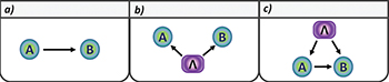
Fig. 3: Directed acyclic graphs (DAGs). (a) Direct influence. An arrow between two different nodes (A and B) represents a causal influence in which A causes an action over B. (b) Common cause. A hidden variable represented by λ generates an influence over two different nodes. (c) Direct and common causation are present simultaneously.
Download figure:
Standard imageAll the ideas and concepts discussed above rely, however, on a classical concept of causality. Inspired by Bell's theorem and the well-known incompatibility of quantum correlations with the usual notion of causality, there has been a surge of results looking for a quantum generalization of these ideas, with the ultimate objective of establishing a quantum theory of causality. On the one hand, there have been a number of different proposals of how to define and treat quantum causal models [26–36]. On the other hand, there is the basic question as to if and how fundamental results in the classical theory of causality should be revisited.
Recently, Ried et al. [26] have shown that it is possible to infer the causal structure from observations alone through a causal tomography. In some cases this implies that one distinguishes between common causes and direct causation, something impossible classically as discussed above. In fact, common-cause mechanisms producing separable states and cause-effect mechanisms implementing entanglement-breaking channels follow the same classical rules and cannot be distinguished. That is, quantum advantage in causal inferring is reached by exploiting entanglement and coherence and was experimentally observed in a photonic experiment [26]. Following that, a quantum optics experiment implementing a coherent mixture of a common cause and direct influence has also been realized [87].
As mentioned before, the instrumental scenario offers a way to distinguish, with observational data, direct causation from common cause. But given that an instrumental inequality can be violated quantum mechanically, is there anything else we should consider? Indeed, as shown in [74], quantum-mechanical effects can lead to an overestimation in the quantification of causal influences. Considering a scenario where all variables are dichotomic, the average causal effect is bounded as [2]  . However, by considering the correlations obtained by measurements on a maximally entangled state it has been proven that the classical bound above would imply that
  even though, if interventions are made, one observes that
  . In other terms, the classical inequality would lead to an overestimation of the causal influence. Finally, it has been shown, both theoretically and experimentally [88], that the instrumental causal model can be used to derive a stronger form of steering.
Future challenges
The interplay between quantum information and the theory of causality is a very recent enterprise with a few different threads. A prominent line of research has been the development of a quantum theory of causality, encompassing the counterintuitive quantum features but also recovering the classical theory in the appropriate limit [26–36]. Another approach has been to remain within a classical theory but allows for relaxations of causal assumptions, which provides insights into the nature of quantum correlations and a natural way of quantifying them [13–15,17–23,89]. Finally, a new fundamental feature that has attracted considerable attention is the coherent superposition of different causal orders [30,33,37–43], yet another quantum phenomenon enlarging even more the quantum supremacy in the processing of information. In fact, as expected, the concepts and tools arising from these initial investigations have already been turned into resources for new kinds of protocols. For instance, quantum effects allow for advantages in causal inference problems [26,32,74,87,90] and superposition of causal orders permits an exponentially advantage in certain communication problems [91–93]. Yet, in spite of these exciting developments, it is fair to say that the application of the causal framework to quantum information problems is still vastly unexplored, specially experimentally and in the context of complex quantum causal networks.
Theoretically, a few challenges are ahead. For instance, the characterization of the set of classical and quantum correlations in causal networks of increasing complexity has seen interesting new results in the last years [53–58] but a more complete picture and more efficient algorithms still lie ahead. Regarding the superposition of causal orders, one of the key open questions is whether quantum mechanics allows for the violation of causal inequalities [94–96], that similarly to Bell inequalities would provide a device-independent framework to the study of indefinite causal orders. Also, to which extension quantum correlations can provide enhancements in causal inference problems remains a topic for further investigations.
From the experimental side, novel fundamental and practically relevant challenges can be pursued which will require more ingredients: several independent sources of states [41–43], classical and quantum communication between the parties [16,24,25,91,93], quantum interventions [24,26] and coherence mixtures of causal structures [87] as well as superposition of causal orders [30,33,37–43].
Acknowledgments
We acknowledge support from John Templeton Foundation via the grant Q-CAUSAL No. 61084 (the opinions expressed in this publication are those of the authors and do not necessarily reflect the views of the John Templeton Foundation). RC acknowledges the Brazilian ministries MCTIC, MEC and the CNPq (grants No. 307172/2017-1, 406574/2018-9 and INCT-IQ) and the Serrapilheira Institute (grant No. Serra-1708-15763). GC acknowledges Becas Chile and Conicyt.
Footnotes
- 1
Following the standard notation, capital letters (e.g., X) denote random variables and lower-case letters (e.g., x) denote the values they acquire. That is, when referring to probabilities we will use the shorthand notation
 .
.