


Abstract
By considering the intrinsic anisotropy, present in almost all magnetic systems, as a perturbation to the usual Zeeman term, we show that the spin-spin dipolar interaction also known as zero-field splitting (ZFS) leads to an extra geometrical phase in addition to the conventional Berry's phase. Furthermore, we suggest some ways to observe the energy shift in electron paramagnetic resonance spectra due to Berry's phase and how we can separate it from the conventional Zeeman Berry's phase.
One of the authors (MM) dedicates this work to the memory of his mother, Djabou Zoulikha, who died on 3 February 2019.
Export citation and abstract BibTeX RIS
Introduction
The evolution of quantum spin systems under time-dependent magnetic field has received renewed attention [1–18]. It is known that under the adiabatic hypothesis, a quantum state picks up an additional phase factor or Berry's phase [1] which turns out to be geometrical in nature in contrast to the well-known dynamical phase factor. The geometric phase has been evidenced by many experimental studies [2–8]. Recently, several proposals have been suggested to use the features of the geometric phase in high technological applications, such as in quantum computing [7–9], in optical information encoding [10] and in many other applications in electronic physics [11]. However, few experimental and theoretical studies have been performed to investigate the effect of some interactions, within a quantum system, on the geometric phase. This is often so because of its weak magnitude compared to that of the dynamic phase on the one hand and on the other hand due to the technical limits. For instance, the effect of the exchange interaction on the geometrical phase was investigated theoretically, within the XYZ Heisenberg model, by Yang et al. [12]. An experimental method based on the Landau-Zener model was developed to measure quantum phase interference in magnetic molecules as well [13].
In magnetism, the famous example of quantum system is that of spin S under the Zeeman term with time-dependent magnetic field (B(t).S) where the geometric phase or Berry's phase manifests after a cyclic and adiabatic evolution as a solid angle  . However, in all magnetic systems with a non-negligible magnetic anisotropy caused either by spin-orbit coupling or a magnetic dipolar interaction [19], an extra term should be added to the Zeeman Hamiltonian, which expresses this magnetic anisotropy or a zero-field splitting (ZFS) as termed in the electron paramagnetic resonance (EPR) language. In this work, we show that the obtained geometrical phase contains two contributions: the well-known Zeeman Berry's phase, as expected, and a new geometrical one, hereafter designated as the magnetic anisotropy Berry's phase. In addition, we propose how both contributions can be experimentally observed and separated.
The simplest Hamiltonian model, sum of the Zeeman and the ZFS term, describing the spin systems including the magnetic anisotropy has the following form:

The two parameters D and E stand for uniaxial and planar anisotropies, respectively. The effect of ZFS on the dynamic phase of isolated transition metals Co2+(S = 3/2), Mn2+(S = 5/2), Fe3+(S = 5/2), embedded in a zinc oxide (ZnO) single crystal is well established and it has been recently studied by EPR spectroscopy [20,21] where the parameters E and D are given. It has been shown that the magnetic anisotropy (ZFS) is maximum when the applied magnetic field B(t) is parallel to the unique axis c of ZnO, and zero, in the first-order approximation, for  (see fig. 1), where
  is the so-called magic angle. Therefore, the contribution of the magnetic anisotropy to the dynamic phase could be easily eliminated from the EPR spectra by setting up the system in such geometrical configuration or by using a magic angle sample spinning (MAS) equipment [22,23].
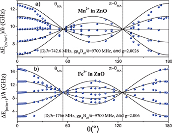
Fig. 1: Variation of the EPR resonance energy as a function of the angle θ of the isolated TM ions in ZnO. (a) Mn2+ with  and angular independent zero-field splitting parameter
  and (b) Fe3+ with
  and
and  (dots) [20,21], with simulation (continuous lines) according to eq. (7) [25].
Download figure:
Standard imageIn order to find the adiabatic evolution of the initial energy eigenstates  , we perform on the eigenstates
  a time-dependent unitary transformation associated with the rotating-frame transformation that brings the magnetic field from an axis defined by the polar angle θ and the azimutal angle ϕ to the quantification axis z [14,15],
in which the spherical variables  and
and  vary slowly in time. The time-dependent Schrödinger equation
  can be mapped to the time-dependent Schrödinger equation
  with the new Hamiltonian

where  .
.
Note that the energy eigenvalues  contain the term
  that causes a shift of the eigenvalues and can be omitted in the adiabatic approximation, because the derivative is proportional to
  and it is therefore negligible. We will show that this term leads effectively to Berry's phase in first order in
  (see eq. [4]). With this, the problem is reduced to solving the Schrödinger equation with the following Hamiltonian
  , where

and the time-dependent coefficients are given by


where  and
and  is the anticommutator.
The instantaneous eigenstates  of
of  can be deduced from
  by the unitary transformation U. In the case of a strong magnetic field and a relatively weak magnetic anisotropy, the
  term varies that very slowly with time so that it can be considered as a perturbation to the Zeemann term.
One can verify that, to the first order in  the expression

is an eigenstate of  , where
  are eigenstate of
  , the normalization constant N(t) is
and with
The geometric phase [1]

leads then to

The second term  is of second order on
  which is neglected in our case. Only the first term is kept and it can be calculated explicitly
thus, the geometrical phase (4) can be calculated explicitly over a period T as

where  .
.
In addition to the conventional Zeeman Berry's phase the above equation brings about a supplementary geometrical phase exclusively attributed to the magnetic anisotropy.
Bruno [24] derived a general expression for Berry's phase (eq. (1)). The simple Hamiltonian to which he applied the theory is different from our Hamiltonian, given that the magnetic field in Bruno's model is along the z-axis while in our case it has an arbitrary direction. In addition, even in the absence of the magnetic field and in the presence of the spinning sample experiment one gets access to Berry's phase [6]. However, the calculation made by Tycko can be compared to Bruno's results because Tycko used a perturbation in  , in contrast our perturbative calculation is
  which cannot be mapped especially in the limit
  where we do obtain the geometrical Berry phase
  while Berry's phase in Bruno's calculation vanishes. The additional phase is topological in nature and as we choose an arbitrary direction for the magnetic field, this corresponds to the group C1 [24] (fig. 1.a in [24]).
Discussion
The analytical expression of the geometric phase (eq. (5)) cannot be solved exactly, because although the two variables  and
and  are not explicitly independent, they are related to each other by their time dependence. For this we limit ourselves to some special cases by considering that θ is almost constant in time, and at first order, we assume it to be time independent.
In this case the geometric phase, after performing the integration over one period of evolution, becomes

We found that the geometric phase (eq. (6)) contains two terms: the first one corresponds to the conventional Zeeman Berry's phase, and the second one is proportional to the uniaxial anisotropy constant D that we call the magnetic anisotropy Berry's phase. Both terms depend on the odd power of the cosines of the angle between the crystal symmetry axis and the effective magnetic field about which the spins are rotating. For systems with a negligible uniaxial anisotropy, the second term will be zero and only the conventional Zeeman Berry's phase remains.
The conventional Zeeman Berry's phase has been observed as energy shift in nuclear quadrupole resonance and analogue expressions are obtained [6]. This contribution vanishes only when the angle between the magnetization axis and the external magnetic field is zero while the magnetic anisotropy Berry's phase vanishes also when the magnetization axis is perpendicular to the external magnetic field. This allows us to distinguish between the two contributions. In addition, the magnetic anisotropy Berry's phase contribution is maximum for the magic angles  at
at  and
and  used in magnetic resonance spectroscopy to eliminate line broadening, e.g., in solid-state nuclear magnetic resonance (NMR).
A substantial shift of the magic angle values can be obtained when including the higher-order terms for energy levels [20]. However, observing the magnetic anisotropy Berry's phase can be achieved by flipping the magnetic field at any angle. In electron paramagnetic resonance (EPR), a paramagnetic sample subjected to an alternating magnetic field superimposed to the Zeeman field shows transitions between Zeeman energy levels according to the selection rule  . As previously mentioned for Mn2+ and Fe3+ ions, these transition energies, within the second-order approximation and in the absence of the geometrical phase, are given by [25]

Equation (7) shows that the EPR transitions for systems with with  vary as (
 except for the transition
  which is independent of θ.
For all EPR transitions energy, the angular dependence of the spin-spin dipolar interaction (ZFS) is an even power of cosines of θ. It oscillates between a maximum located at 0 and π and a minimum located at  or inversely (see fig. 1), while vanishing at
  and
and  . This is shown in fig. 1, which depicts the experimental angular dependence of the resonance field for Mn2+ and Fe3+ ions in ZnO for a fixed microwave frequency, together with the simulated behavior [20,21] according to eq. (7) [25].
Using eq. (6), Berry's phase of these two paramagnetic systems may be expressed as

where  .
.
The shift in the geometrical phase will correspond to a shift in the transition energy given by  [16]. These energy shifts due to the geometrical Berry's phase contribution, using the experimental values of D [20,21] and
  [22], where
  is the MAS rotation frequency, are presented in fig. 2. It is shown that this contribution is very small compared to the transitions energies given by eq. (7) (four orders of magnitude smaller). Such contribution will be difficult to observe directly, contrary to the nuclear quadrupole resonance experiment [6] where the shift in energy is comparable to the transition energies.

Fig. 2: Simulated evolution of the energy shifts due to the geometrical phase as a function of the angle θ for fixed rotation frequency  , for TM ions in ZnO; (a) Mn2+ with
  and
and  and (b) Fe3+ with
  and
and  .
.
Download figure:
Standard imageTo separate the geometrical contribution, we calculate the difference in the transition energies at angle θ and at angle  . Doing so allows removing the contributions of the even powers of the cosines, i.e., the dynamical contribution (eq. (7)), so that only the odd powers remain as discussed above (see fig. 2). In addition, to get the lonely Zeeman Berry's phase we add
  and
and  , while to get the magnetic anisotropy Berry's phase we subtract
  and
and  .
.
The energy shifts due to the magnetic anisotropy Berry's phase normalized by a factor  are represented in fig. 3. As previously mentioned, this contribution is maximum at the magic angle (see eq. (6)).

Fig. 3: Energy shift due to the magnetic anisotropy Berry's phase normalized by a factor  (see text). The dashed lines indicate the magic angles.
Download figure:
Standard imageNote that switching B to  is equivalent to the transformation
  procedure. The advantage is that it does not include any experimental uncertainty. This is currently used in X-ray magnetic circular dichroism (XMCD) [26] or by using the spin-echo method in pulsed electron paramagnetic resonance for
  , where the dynamic phase can be entirely eliminated keeping only the geometric phase contribution [7,8,16].
To complete this observation, note that from symmetry arguments and due to the fact that the Zeeman term is linear in spin and by consequence it changes sign under time-reversal symmetry T, the anisotropy term, caused either by spin-orbit coupling or by the spin-spin dipolar interaction, is invariant by time-reversal symmetry. Therefore, we may keep the magnetic field and the angle fixed while switching the spinning direction of the sample (Onsager relations [27]).
Conclusion
In this letter, we showed that, in a magnetic system with a non-negligible magnetic anisotropy, subject to an alternating magnetic field, Berry's phase will show up as a shift of the resonance of the EPR spectra. This modification is caused by the conventional Zeeman contribution as well as by an additional contribution due to the magnetic anisotropy Berry's phase. Although this contribution is too small to be commonly observed according to the usual spectra linewidths, we proposed a way to observe and to separate each geometrical contribution. As a proof of concept, we used the measured values of ZFS of Mn+2 and Fe3+ ions diluted in a ZnO matrix. Given a magic angle spinning of the sample the proposed procedure allows the measurement of the magnetic anisotropy Berry's phase through EPR experiments, as previously discussed by Goldman [17].
Acknowledgments
The French-Algerian PHC TASSILI program (CMEP-12MDU861) is gratefully acknowledged for a financial support to the present work. KB would like to thank Dr. Yahia Saâdi (University of Setif 1) and Dr. Jérôme Tribollet (University of Strasbourg) for their helpful discussions.