

Abstract
X-ray computed tomography (CT) reconstruction suffers from beam-hardening artefacts caused by the polychromaticity of virtually all lab-based X-ray sources. A method to correct for beam-hardening is a direct, pixel-wise signal-to-thickness calibration (STC). We compare reconstructions of conventionally flat-field corrected as well as STC preprocessed measurements of various samples performed on a commercial microCT device based on a flat-panel detector. We show that a good estimate between the transmission signal and the respective material thickness can be given by multiple exponential functions. We further compare the exponential interpolation approach to a hyperbolic model, which reduces the number of necessary calibration measurements significantly. Our method shows that typical beam-hardening artefacts like cupping and filling can be almost completely suppressed and a significant contrast increase is gained. The method can be applied with little additional calibration and computation effort and allows shorter acquisition times since beam filtration can be reduced or omitted.
Export citation and abstract BibTeX RIS

Published by the EPLA under the terms of the Creative Commons Attribution 3.0 License (CC-BY). Further distribution of this work must maintain attribution to the author(s) and the published article's title, journal citation, and DOI.
Introduction
X-ray computed tomography (CT) is an invaluable 3D imaging technique with countless applications in biological, medical and material research and is widely used in clinical routines for diagnosis as well as in industrial applications for non-destructive testing. In its basic form it delivers a 3D distribution of the attenuation coefficient μ of a sample. The attenuation of X-rays by a homogeneous material of length x is described by the well-known Lambert-Beer law:

where I0(E) is the intensity at an energy E of the impinging beam and  is the energy-dependent linear attenuation coefficient of the material. By measuring the attenuated signal I(x, E) in form of 2D X-ray projection radiographs at different angles around the sample and the respective I0 in a flat-field image a 3D distribution of attenuation coefficients can be calculated by tomographic reconstruction algorithms (e.g., filtered backprojection, FBP). A great difficulty in the practical realization of CT systems is introduced by the polychromaticity of common laboratory-based X-ray sources. The relation between the transmitted thickness and the measured intensity deviates significantly from the Lambert-Beer law as the attenuation in the polychromatic case is described by

Increasing attenuation cross-sections towards lower energies cause an increase of the mean energy of the spectrum as the beam passes through the material, which is called beam-hardening. Consequently, regions toward the edges of a measured sample appear more attenuating than the interior since the latter is traversed with a harder X-ray spectrum. In the reconstructed 3D volume beam-hardening becomes apparent in an artificial radial decrease in grey values from the periphery of the measured object to its center [1]. Furthermore, dark or light streaks between and around high attenuating objects like bone can be observed [2].
To suppress this deficiency the X-ray beam is often filtered by metal sheets to get rid of the soft fraction of the beam [3,4]. As the photon flux, also for higher-energy X-rays, is significantly reduced upon filtering, the growing noise level is disadvantageous. In order to achieve comparable photon statistics it is possible to increase the scan time or the beam intensity. However, the latter generally results in an increase of the focal spot size and hence a decreased spatial resolution [5].
Further, several post processing methods prior to reconstruction can be applied to correct for beam-hardening artefacts. Usually the polychromatic ray sum  is mapped to its monochromatic equivalent by assuming some linearization model [6]. The determination of suitable coefficients for a linearization function is not straightforward since it depends strongly on the used X-ray tube parameters, filtration, scanned material composition and thickness as well as the detector type and pixel response. The commonest model is some polynomial correct function of degree 2 or 3 for weakly absorbing [6] and degrees up to 8 and higher for strongly absorbing samples [7]. Nowadays commercial CT devices are provided with proprietary reconstruction software which frequently offers such an implementation of a polynomial correction. However, it is usually not well documented and rather designed to provide some fast ad hoc solution by adjusting a single user-defined parameter on a trial and error basis and evaluating the beam-hardening suppression result by eye.
More appropriate polynomial coefficients can be derived from the used X-ray spectrum [8,9] as well as from experimental calibrations [10,11] or virtual calibrations which usually involve a segmentation of an initial reconstruction [12–15]. Furthermore, an iterative approach can be used to determine the coefficients by minimizing user defined artefacts [16]. The main disadvantages, on the one hand, are time-consuming reference measurements of usually a single material with similar attenuation characteristics as the scanned sample and the required a priori information about the spectrum. On the other hand, segmentation-based and iterative methods generally involve a greater implementation effort and come with high computational expenses. Moreover, since beam-hardening has also been shown to have an impact on dimensional measurements, it can complicate or even preclude an accurate segmentation of the initial beam-hardening affected reconstruction [17–19].
An alternative experimental calibration routine to the mapping of the monochromatic ray sum is a direct interpolation of the transmission signal depending on the thickness of a material which is referred to as a signal-to-equivalent-thickness calibration (STC) [20]. This method has been demonstrated for photon counting and flat panel detectors using local exponential and linear interpolation functions [20,21].
In this work we propose a hyperbolic interpolation function which fits the transmission signal response in a wide thickness range. In particular, it reduces the necessary number of calibrated thicknesses significantly and simplifies the processing procedure compared to local interpolations based on exponential functions. Further, we apply this method to a commercial microCT equipped with a flat-panel detector and show that the pixel-wise STC calibration method can be easily implemented with great benefit even when the sample materials deviate from the reference calibrator material.
Interpolation methods for STC
Despite the imperfections originating from a potential divergence of calibration and sample materials, the main disadvantage of STC-based beam-hardening correction is the time-consuming reference measurement, which has to be repeated for every unique scan configuration (X-ray tube material, detector type, energy, exposure time, etc.). The number of measured calibration points depends strongly on the interpolation model used in the STC procedure. In case of polynomial functions, high degrees are needed for a proper correction of strongly absorbing samples like aluminum or steel [7]. Fitting such high-degree polynomial functions to actual transmission data is difficult, since the interpolation tends to oscillate between measured points particularly at the interval edges (Runges phenomenon) and strongly approaches positive or negative infinity after the last interpolation point. Hence, fitting of high-degree polynomials is only useful and robust when many transmission measurements of the entire thickness range of the actual CT scan are made. An alternative interpolation model, which avoids the problems of the high-degree polynomial approach, assumes that in each calibration point the signal-to-thickness conversion function can be approximated by local exponential interpolations (LEI) with offset [20]:

with the constant parameters  ,
,  and
and  . Figure 1 shows piecewise fits of such exponentials into three neighbouring points, respectively, for a calibration measurement of an aluminum alloy (AlMg3). This model can further be extended by applying the logarithm to the data prior to the interpolation [21]. The advantage of the linearization is that the local exponential functions can then be replaced by linear interpolations which use fewer constants and are also easier to implement. However, since a piecewise fit intrinsically requires more calibration points compared to a single interpolation function and also involves increased computational effort, we found that a hyperbolic function of the form

describes the signal-to-thickness response across a wide thickness range. In this semi-empirical model the three parameters  ,
,  and
and  do not have a fundamental physical meaning but can be easily determined from a significantly reduced number of transmission measurements. This interpolation will be referred to as the global hyperbolic interpolation (GHI) since in contrast to the LEI method it covers the whole range of thicknesses by a single fit function. Exemplary fits based on the GHI method are shown in fig. 2 for multiple materials and energies in order to demonstrate the interpolation performance for different curve shapes. Here, only the four calibration points which are indicated by the filled markers were used for the interpolations, respectively.
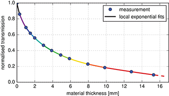
Fig. 1: Signal-to-thickness calibration (STC) based on local exponential interpolations (LEI) for a random pixel of a flat-panel detector. The coloured connecting lines correspond to the piecewise fit of three neighboring calibration points, respectively.
Download figure:
Standard image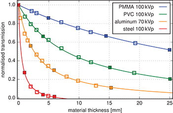
Fig. 2: Signal-to-thickness calibrations (STC) based on a global hyperbolic interpolation (GHI) for multiple materials and a random pixel of a flat-panel detector. Note that only the calibration points indicated by filled markers were used for the fit.
Download figure:
Standard imageA comparison of the GHI and the LEI with the measured data points is shown in fig. 3 for the different materials. The measurements are covered very well by the piecewise interpolations, whereas an oscillation of the GHI residual around zero is visible. This suggests that limitations of the GHI model occur with calibration curves with a very steep decrease of the signal at small thicknesses and a very flat decrease at larger thicknesses as the model is not capable to cover both features accurately at the same time. These cases can be avoided by adjusting the measurement parameters (higher tube voltage or/and beam filtration) according to the respective sample properties. Another issue of the GHI model recognizable in the steel data (fig. 2) is a possible extrapolation of transmission values below zero, which is physically unreasonable. However, such extrapolated thicknesses are not used for the reconstruction since measured transmission values are always positive.
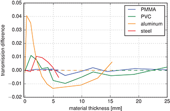
Fig. 3: Residual (difference model—measurement points) of the global hyperbolic (GHI, solid lines) and the local exponential (LEI, dashed lines) interpolation functions for the data in fig. 2.
Download figure:
Standard imagePractical realization
In order to evaluate the practical feasibility of the GHI method for beam-hardening correction, signal-to-thickness calibration measurements were performed on a GE phoenix v∣ tome∣ x s 240 microCT device using sheets of an aluminum-magnesium alloy with a magnesium content of approximately 2–4% (referred to as AlMg3 in the following). The calibrator thicknesses were 0, 0.30, 1.0, 1.5, 2.0, 3.0, 3.9, 4.9, 5.9, 7.9, 9.8, 12.8 and 15.3 mm. For each aluminum thickness a calibration image was obtained by averaging 30 projections acquired with a tube voltage of 70 kVp, a tube current of  and an exposure time of 1 s, respectively. No additional beam filtration was applied. For a comparison of the LEI and GHI models, both methods were applied on the same calibration data. For the LEI method, calibration curves were obtained by locally fitting three neighboring points according to eq. (3), respectively (see fig. 1). For the GHI method, only the four points at 0, 2.0, 5.9 and 15.3 mm aluminum thickness were used for a global fit according to eq. (4) (see fig. 2). Due to the individual detection efficiency of flat-panel detector pixels, the calibration curves for both interpolation models were acquired pixel-wise. For each individual pixel, the actual calibrator thicknesses were adjusted to the slightly increased effective thicknesses traversed by the cone beam. Several samples with varying degrees of deviation from the calibrator material composition were considered. First, a phantom composed of one filled (aluminum-copper alloy) and two hollow (aluminum-magnesium alloy) rods was examined. Furthermore, an aluminum electrolytic capacitor with a plastic coating, a concrete drilling core and a bone sample, were investigated. According to the guidelines given in [22], the bone sample was placed in a plastic vessel and submerged in a liquid medium (ethanol). The scan parameters for the different samples were identical to those of the calibration measurement and the maximum sample thicknesses were all within the calibrated thickness range from 0 to 15.3 mm. FBP reconstructions were performed from either 1001 (aluminum phantom, capacitor, drilling core) or 1201 (bone sample) projections after a conventional single flat-field correction (FFC) as well as after a signal-to-thickness calibration using the LEI and GHI model, respectively. For all samples, the AlMg3 alloy was used as the calibration material.
Results and discussion
The results for the aluminum phantom are depicted in fig. 4(a)–(c) in form of normalised cross-sections through the reconstructed volumes. Lineplots along the coloured lines in fig. 4(a)–(c) are shown in fig. 4(d) and (e) for the hollow and filled cylinders, respectively. The mean over several cross-sections was taken for the lineplots to suppress the influence of noise. The FFC data clearly suffers from strong beam-hardening artefacts. On the one hand, cupping in all three cylinders can be observed. On the other hand, bright streaks connect the outer parts of the three cylinders, which is clearly visible in the lineplot in fig. 4(e). Another typical beam-hardening consequence is the artificial filling of empty regions that are enclosed by a material. This can be observed in the central regions of the hollow cylinders, which are calculated to values slightly higher than zero. Similar beam-hardening artefacts can be observed in the other three samples which are depicted in fig. 5–7. Here, the most pronounced artefact affecting the image quality is cupping which goes hand in hand with a significant contrast reduction.

Fig. 4: A phantom composed of three aluminum cylinders reconstructed with a conventional flat-field correction (a), signal-to-thickness calibrated data using the local exponential interpolation (LEI) (b) and global hyperbolic interpolation (GHI) (c) approaches and lineplots for the hollow (d) and filled (e) cylinders. The calibrated reconstructions eliminate cupping, streak and filling artefacts and, therefore, allow for a differentiation of the two different aluminum alloys in the phantom.
Download figure:
Standard image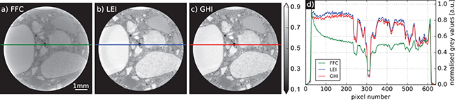
Fig. 5: Concrete sample reconstructed with a conventional flat-field correction (a), signal-to-thickness calibrated data using the LEI (b) and GHI (c) approaches and respective lineplots (d). The suppression of cupping results in significant contrast enhancement between the concrete compounds.
Download figure:
Standard image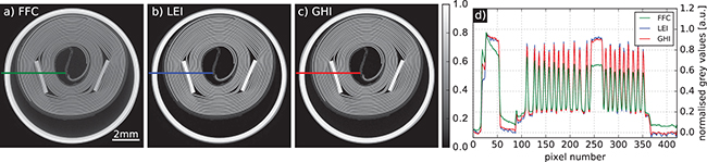
Fig. 6: Aluminum electrolytic capacitor reconstructed (a) conventionally (FFC) and using the signal-to-thickness calibration with the LEI (b) and GHI (c) approaches. The coiled electrodes connected to both contacts are clearly recognisable. Lineplots (d) of STC reconstructed data show that even the alternating anode and the cathode electrodes are distinguishable due to slightly different aluminum purities typically used for the electrodes.
Download figure:
Standard image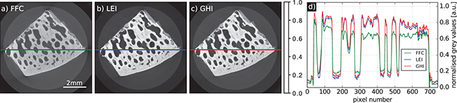
Fig. 7: Trabecular bone sample reconstructed with a conventional flat-field correction (a), signal-to-thickness calibrated data using the LEI (b) and GHI (c) approaches and respective lineplots (d). A significant contrast enhancement is achieved although the bone sample is surrounded by materials which have significantly different X-ray attenuation characteristics compared to the calibrator material.
Download figure:
Standard imageIn the LEI and GHI reconstructions, however, cupping as well as the streak and filling artefacts are eliminated almost completely in all investigated samples. Furthermore, a significant contrast enhancement can be observed. Thus, a grey-value–based separation of the two different aluminum alloys in the cylinder phantom as well as the two coiled capacitor electrodes is enabled, which is almost impossible in the standard FFC reconstruction. Although the GHI reconstruction was performed using a significantly reduced number of calibration measurements it is very similar to the LEI reconstruction. The latter even shows some slight grey-value variations across the cylinders in the phantom where the GHI reconstruction is more homogeneous. The slight over-correction of the filled cylinder in the GHI data is probably due to an overestimated thickness as the aluminum-copper alloy is more attenuating than the AlMg3 used for calibration. By contrast, the LEI reconstruction features a small grey-value oscillation in the lineplot in fig. 4(e). A similar effect can be observed in the result for the drilling core sample. Here, the LEI calibration introduces a faint ring at the outer part of the sample. This is due to the fact that the LEI calibration is realised with piecewise fits that may feature non-smooth transitions into each other, especially when an insufficient amount of calibration points is available. On the contrary, the GHI method yields a single, smooth calibration curve. Our calibration results indicate that the calibrator and sample material do not have to be explicitly the same. The main requirement is a similarity in terms of their X-ray attenuation characteristics. Furthermore, the sample can also be composed of multiple materials as long as they do not vary too strongly in attenuation. Thus, despite of the diverse concrete composition in the drilling core sample, a significant image quality improvement is achieved. Also for the trabecular bone sample, the calibration yields a cupping correction and contrast enhancement although the aluminum-equivalent bone is surrounded by ethanol and a plastic vessel.
Conclusion
In X-ray imaging, the signal-to-thickness calibration is an experimental data linearization approach. In this work we presented the impact of such a calibration on the image quality in computed tomography using a flat-panel-detector–based microCT device. Our results show that beam-hardening artefacts like streaks, cupping and filling can be effectively eliminated by a pixel-wise calibration. Moreover, the precise knowledge about the material composition of the sample is not necessarily required as long as there is no extreme variation in attenuation among the individual sample components. Therefore, for a wide variety of samples a single calibration material with similar attenuation characteristics can be used for a reasonable calibration result. Finally, we showed how the calibration time, which is a major disadvantage of the STC method, as well as the computational effort can be significantly reduced by using a simple hyperbolic interpolation model.
Acknowledgments
We acknowledge financial support through the DFG Gottfried Wilhelm Leibniz program.