

Abstract
We consider a one-dimensional (1D) array of coupled quantum harmonic oscillators of arbitrary size in the presence of staggered losses. The dynamics of the system is analyzed thoroughly, through exact solutions in which exceptional points (EPs) are found to greatly impact the system dynamics. In particular, different dynamical regimes arise due to the progressive emergence of EPs varying the interaction strength, also allowing for single frequency emission of all array components. Signatures of these regimes are found in the decay dynamics of the system, in the transmission and fluctuation spectra, and in the emergence of frequency windows where resonant absorption and emission are strongly inhibited because of interference effects.
Export citation and abstract BibTeX RIS
Introduction
Coupled open quantum systems display dynamical features which cannot be inferred solely by the unitary dynamics of the system nor by the dissipative dynamics of its uncoupled units. Instead, even in the presence of local dissipation, the interplay of coherent interactions and decays needs to be considered as a whole to explain the dynamics of the system. Recently, effective non-Hermitian models have been explored in this context. Contrary to Hermitian (closed) systems, non-Hermitian ones can show exceptional points [1–9]. An exceptional point (EP) is a point in parameter space at which two or more eigenvalues and their respective eigenvectors of the Hamiltonian coalesce [1,2]. Such degeneracies are ubiquitous in open systems that exchange energy with their surrounding environment [3] and are at the heart of a wide variety of intriguing phenomena observed in different physical settings, such as parity-time symmetry breaking [4–8,10–13], extreme sensitivity to perturbations [14,15], chiral dynamics for adiabatic EP encircling [16–19], anomalous quantum decay [20,21], and topological phenomena [22]. In particular, dissipation can dramatically change the way a composed system oscillates: while in closed systems any coherent coupling modifies the eigenfrequencies, dissipation can give rise to a far richer variety of phenomena. For instance, a dissipative system can oscillate at the bare intrinsic frequency of its units in spite of their mutual coupling. This effect can be related to the normal mode splitting earlier predicted for atoms interacting with vacuum in cavity [23,24] and observed in several platforms (see [25,26] and references therein). Dissipation-induced frequency degeneracy can influence also the response of the system as observed in emission and absorption spectra. Indeed, excitations with the same frequency can interfere destructively yielding transparency windows, in which the system does not react to resonant driving [27–31], as well as frequency windows in which thermal emission is strongly inhibited [32]. The interplay between interactions and damping in composite systems, besides modifying the decay of excitations to the continuum introducing polynomial corrections to the typical exponential decay [20,21], distributes the decay rates of modes of the system leading to phenomena like superradiance [33] and synchronization [34,35], as well as the possibility of decoherence-free subspaces [36–38].
In this work, we study the interplay between coherent dynamics and dissipation arising independently on each unit of composite systems when we allow for different damping rates. We consider a 1D array of coherently coupled identical bosonic systems each of which dissipates into its own independent environment with staggered rates. This kind of model is of relevance in the context of quantum technologies, where systems made of coupled resonators are ubiquitous, as, for instance, mechanical [32,39,40] and optomechanical [41,42] arrays, coupled photonic modes [43], and arrays of superconducting microwave resonators [44]. Interestingly, the 1D array system with staggered dissipation shows a set of EPs in both first and second moments dynamics which separate different dynamical regimes characterized by a rich phenomenology, such as qualitative distinct temporal behaviors towards the stationary state and the emergence of interference effects in the transmission and fluctuation spectra. Quite remarkably, the EP entails the possibility of achieving a regime where all system components oscillate at the same (bare) frequency for any initial condition, in spite of coherent couplings. Finally, we briefly establish connections with phenomena already familiar in the literature and observed in different physical systems, such as Fano interference and electromagnetic-induced transparency (EIT) [45].
Model
We consider a 1D tight-binding chain of quantum harmonic oscillators with uniform frequencies  and tunneling rates λ. The units are weakly coupled to independent baths in a staggered way, such that the system is composed by N cells of two dissipative modes each. The Hamiltonian and master equation in Born-Markov approximations describing the system in the rotating frame with
  read (
 )
)


where ![$\mathcal{D}[\hat{o}]=2\hat{o}\hat{\rho}\hat{o}^\dagger-\hat{o}^\dagger \hat{o}\hat{\rho}-\hat{\rho}\hat{o}^\dagger \hat{o}$](https://content.cld.iop.org/journals/0295-5075/127/2/20001/revision1/epl19774ieqn4.gif) . Notice that in principle we consider general out-of-equilibrium environments in which the rates
. Notice that in principle we consider general out-of-equilibrium environments in which the rates  and
and  do not satisfy necessarily detailed balance. Moreover, the local character of dissipation is well justified when the coupling between units is small
  [46].
[46].
Dynamics of the first moments
Let us start our analysis considering the first moments, whose dynamics can be understood as the superposition of N independent pairs of interacting modes. Each of these pairs, from now on referred as k-modes, displays two dynamical regimes separated by an EP. These regimes are characterized by the number of dynamical frequencies of the system and the way it decays (fig. 1). The equations of motion of the first moments read


with ![$n\in[1,N]$](https://content.cld.iop.org/journals/0295-5075/127/2/20001/revision1/epl19774ieqn8.gif) ,
,  , and
, and  the Kronecker delta. Equations (3) and (4) can be conveniently written in matrix notation as
  , where
  and
and  represents a possible additional driving term.

Fig. 1: (a) Real and imaginary parts of  are shown as red solid lines and blue dashed lines, respectively. (b) Real part of
  as a function of time. In magenta
  in which all k-modes are in the single-frequency regime except for k1. In green
  in which all modes are in the two-frequency regime except for those of k3. In blue
  and all modes are well into the two-frequency regime. The initial condition corresponds to excitation of the first site solely. In both panels N = 3,
  and
and  .
.
Download figure:
Standard imageExceptional points
Let us introduce the vector of moments via the orthogonal transformation  , where
  contains the k-modes
  defined by


with  ,
,  and similarly for
  . This transformation preserves the commutation relations because
  and
and  (
( ), as one can readily show. Then
  with
with  and
and

with  . The eigenvalues of the whole system are obtained by diagonalizing the
  blocks and read

with  . We denote the eigenvalues real and imaginary parts as
  and
and  , respectively (fig. 1(a)). We obtain that, as the coupling λ is varied, below a certain threshold the eigenvalues are real, while above they become complex. When the imaginary parts vanish (moving from the rotating frame to the lab one) all units oscillate at their bare frequencies,
  , in spite of their mutual interactions. This is in stark contrast to what one observes in the corresponding closed system where, for any coupling strength, the eigenfrequencies differ from the intrinsic frequency
  . At the symmetry breaking threshold point the square root in eq. (7) vanishes and the two eigenvalues with the corresponding eigenvectors coalesce [1,2]. This point is thus an EP, at which
  (and thus
  ) becomes non-diagonalizable. Therefore, our system displays N EPs (fig. 1(a)), one for each kl. The EPs separate different regimes in which the number of frequencies varies from 1 to 2N, a feature that cannot be observed for any closed or homogeneously dissipating system. Indeed, in the case of balanced loss rates
  , the bath would only introduce a uniform dissipation decay, while the frequencies would depart from
  and be modified as in the absence of the environment.
Decay dynamics
To study the decay dynamics near an EP, we proceed to solve directly the block-diagonal system of equations using the Laplace transform method. The equations for the k-modes are


Solving their Laplace transformed version we obtain in the s-domain:


and the initial condition given by  . The poles
  correspond to the eigenvalues of
  , which display an EP in each k-block at
  . Here, as well as in the scattering matrix, an EP appear as a double pole, which makes clear the emergence of polynomial deviations from the typical exponential-decay behavior. From eqs. (7), (10) and (11) we identify two dynamical regimes for each k-mode, separated by an EP. i) Single-frequency regime
  : we have two different real poles and no oscillations (in the rotating frame). ii) Exceptional point
  : we have a real second-order pole, yielding polynomial corrections to the exponential decay without oscillations. iii) Two-frequency regime
  : we have two different complex poles, yielding oscillations with equal damping. In the time domain the dynamics in each regime read as follows.
i) Single-frequency regime:
where  is the Heaviside step function. Notice that in all cases the solution for
  is obtained from the one of
  by exchanging the labels
  and the initial conditions. In this regime the poles are real and read as
  .
.
ii) Exceptional point:

iii) Two-frequency regime:

Here the poles are complex, and the imaginary part is  .
.
The solution in the site basis is obtained reversing the orthogonal transformation, i.e.,  (eq. (5)). Hence, in the site basis, the local dynamics is a combination of the different k-modes ones. As anticipated, the number of frequencies at which the modes can oscillate change depending on the regime. Below the first EP, the modes oscillate mono-chromatically, despite the finite coherent coupling. This region of monochromatic evolution of all units occurs in a parameter window that depends on the size of the system: in the limit of large N the decay contrast
  is required to overcome coupling, while for just a pair of oscillators one would get a smaller contrast
  .
.
When the previous condition is not fulfilled, for instance increasing the coupling λ between elements, more k-modes enter in the two-frequency regime and, in the site basis, up to 2N frequencies are observed (fig. 1). At the EP, the first moments present an exponential-power-law decay [21]. The exponent of the polynomial corrections can be at most h − 1, where h is the number of eigenvalues that coalesce, i.e., the order of the EP. For higher-order EPs, more frequencies merge at the EP, and the variability in the number of frequencies displayed by the system is magnified. This could occur in our system when periodically modulating losses over larger cells. Finally notice that, despite the peculiar behavior at the EP and its singular spectral character, the solutions are continuous in the transition from one regime to the other, as also observed in other physical contexts (see below).
Driven system and transmission spectrum
Let us now move to the case of a system with driving, i.e., non-zero  . The details on the general solutions are provided in the supplementary material Supplementarymaterial.pdf (SM). Here we focus on the particular case in which we only drive one mode with an oscillatory input of frequency
  , i.e.,
  with
with  . Then in the k-basis the driving terms read as
  and
and  , where α is the driving strength and
  characterizes the input channel. Assuming vanishing initial conditions (SM), the solution in the s-domain is given by


Notice that the only pure imaginary pole is  . Hence, in the transient dynamics towards the steady state, the different dynamical regimes are manifested in the dynamical response of the system to the oscillatory drive through
  . In fact, in the steady state, the intrinsic dynamics of the system appears through the residue of
  , which leads to the following stationary amplitudes for the k-modes:


It is useful for the discussion that follows to particularize the expression for  in the two dynamical regimes, making use of the explicit expression of
  . In the single-frequency regime we have

while in the two-frequency regime we have
We can find signatures of these dynamical regimes in the transmission spectrum of the driven mode. Within the assumption that the system is driven through the environment described in eq. (2), the input-output relation for the driven mode is just  , where
  and
and  [47]. The transmission coefficient is defined as
  , which in the steady state reads

It is clear that the different regimes described explicitly by eqs. (19) and (20) translate into different behaviors of the transmission spectrum. This can be observed in fig. 2, in which we plot eq. (21) (red solid lines) for three different cases: in (a) and (b)  all k-modes are in the single-frequency regime, in (c)
  (only the modes of k3 are in the single-frequency regime), while in (d)
  (all k-modes are well into the two-frequency regime).
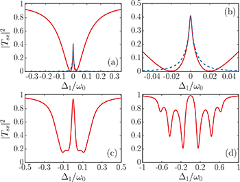
Fig. 2: Spectral transmission  for mode
  driven at frequency
  with
with  . (a)
. (a)  . (b) Zoom-in of the interference window. (c)
  and (d)
  . In all cases N = 3,
  , and
, and  . Red solid lines: exact expression. Blue dashed lines: approximate expression.
Download figure:
Standard imageA surprising feature of this spectrum is that, in cases (a), (b), (c), the system displays a transparency window centered at  , despite the presence of k-modes of this frequency that naively should resonate perfectly with the driving. This can be understood by analyzing the stationary amplitude of the k-modes in the single-frequency regime. Indeed, from eq. (19) we see that these amplitudes have two contributions that interfere destructively, both centered at the same frequency but with different decay rate. In fact, for weak coupling
  , large disparity
  , and near the resonant driving
  , we can approximate the transmission spectrum as

where we have made the replacements  ,
,  and
and  , accordingly to the above approximations. In fig. 2(a) and (b) we compare this approximate expression (blue dashed lines) with the exact one, finding good agreement in the expected region. Thus, eq. (22) enables us to clearly visualize the Lorentzian transparency window that emerges in the single-frequency regime. Notice that the height and width of this window increase with the coupling strength, as is clear from this expression and panels (a) and (c). The interaction-induced transparency windows have been already observed in different systems and configurations, as, for instance, in optical resonators [27,28] or optomechanical systems [29–31], and can be ultimately traced back to the rather general phenomena of Fano interference and EIT [45,48].
In the two-frequency regime we find the more intuitive result that each k-mode contributes to the transmission spectrum with a Lorentzian absorption line centered at its frequency (see eq. (20) and fig. 2(d)). In this case it is no surprise that the system is fully transparent at  as there are no k-modes resonant to this frequency. Furthermore, a distinctive feature of our system is that it can work in both regimes simultaneously, as in case of fig. 2(c), in which there is the transparency window due to the k3-modes, but there are also two double-peak Lorentzian absorption lines due to the other k-modes. Finally we observe that the transmission coefficient is continuous along the different dynamical regimes, as follows from eqs. (17) and (21) and the fact that
  are continuous. This is in spite of the singular character of the EPs and in accordance with what we have commented previously.
Dynamics of the second moments
Let us now consider the dynamics of the second moments. We will first discuss the general method to solve the set of coupled equations of motion, showing that in general the dynamical scenario becomes more complex. Nevertheless, the same dynamical regimes will be shown to emerge in some special instances. Then we will compute the stationary state, which will be used to analyze signatures of the EPs in the fluctuation spectrum of the system.
Equations for the second moments
The system of differential equations describing the dynamics of the second moments is divided into two uncoupled blocks: a homogeneous set of equations for the dynamics of all possible moments of the kind  ,
,  ,
,  and their Hermitian conjugates, and an inhomogeneous system of equations set for the dynamics of all terms of type
  ,
,  ,
,  together with their conjugates. The inhomogeneous block of equations (the only relevant part in our analysis) can be readily written from eqs. (1) and (2) (as done in the SM) and its structure is that of a square lattice with four different sites per unit cell, fig. 3(a). This suggests that the system of equations can be brought to a block diagonal form by means of the orthogonal transformation
  generalized to a 2D lattice. Thus, two wave vectors are needed, kx and ky, and each block reads


where we have defined  ,
,  ,
,  , and
, and  and we have used the dot in place of the time derivative. Hence, we have transformed a general set of 4N coupled differential equations into a reduced one of only 4 coupled equations, which can readily be solved. In the following we calculate explicitly the general solution of eqs. (23)–(26) in the cases in which EPs are observed and the stationary state of the system.
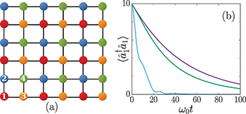
Fig. 3: (a) Lattice model for N = 3, red dots (1)  , green dots (4)
  , blue dots (2)
  , orange dots (3)
  . (b) Population of the first site for
  (magenta),
  (green), and
  (blue), with N = 3,
  ,
,  ,
,  ,
,  ,
,  .
.
Download figure:
Standard imageEPs in the second moments
Let us take an initial condition that is uniform along each sublattice,  ,
,  and
and 
 , and analyze the evolution of the population of each mode. Using the orthogonality properties of the canonical transformation defined in eq. (5), we can show that in the k-basis the initial condition reads as
  ,
,  and the rest of the second moments zero. Then all sectors of eqs. (23)–(26) with
  vanish identically at all times. The solutions in the k-basis and in s-domain are


with  ,
,  and
and  . As before, the dynamics of the second moments in the site basis can be obtained transforming back to time domain and writing
  ,
,  and
and  . From eqs. (27)–(29) it is clear that
  ,
,  and
and  , display the same dynamical regimes as the first moments, and, thus, the time evolution of the second moments presents also the characteristic features of each regime: only one frequency (
 ) and multiple decay rates in the single-frequency regime, polynomial corrections in the decay just at the EP, and multiple frequencies with the same decay rate in the two-frequency regime. Indeed, here at the EP three poles coalesce, which makes the polynomial corrections to be quadratic in time. Examples of the emergent dynamics in the site basis are plotted in fig. 3(b).
Stationary state
Two key observations are needed to find the stationary state: only the equations for the blocks with  have sources, and all blocks described by a homogeneous system of equations go to zero in the stationary state. Then, setting the time derivatives of eqs. (23)–(26) to zero and solving the algebraic equations, we can obtain the non-zero moments in the stationary state. In this way the obtained stationary second moments recombined in the site basis read as


and  follows from eq. (32) exchanging the labels
  . In case that sublattice effective temperatures are the same,
  , we recover the familiar scenario, induced by the presence of local losses in the Lindblad equation (2) in which the only non-zero moments are
 . However, in the general case off-diagonal terms are also present, which can lead to the presence of correlations in the stationary state of the system. Indeed, as the master equation (2) is bilinear in the mode operators, if the initial state is Gaussian the stationary state is Gaussian too, and we can fully describe it constructing the covariance matrix, σ, from the above solutions [49], which displays the characteristic block diagonal structure of our system:
  . Notice that even though the difference in sublattice effective temperature can induce non-local correlations in the stationary state, such correlations are not related to the transient dynamics and to the presence of EPs and will not be reported here.
Emission spectrum
As described by eq. (2), our open quantum system is subjected to the influence of the environments, which cause fluctuations and fluxes of energy. These effects can be characterized by means of the emission and absorption fluctuation spectrum which can be computed from two-time correlation functions in the stationary state [47,50,51]. In this section we show that in these quantities, we also find signatures of the different dynamical regimes, and thus of the presence of EPs.
In fig. 4 we plot the emission spectrum ![$S(\Delta)=\textrm{Re}[\langle \hat{a}_1^\dagger\hat{a}_{1}(\Delta)\rangle]$](https://content.cld.iop.org/journals/0295-5075/127/2/20001/revision1/epl19774ieqn151.gif) vs. the coupling strength for a chain of six elements (N = 3) and with
vs. the coupling strength for a chain of six elements (N = 3) and with  . This quantity is defined from
  with
with  , which can be computed from the previous results following the quantum regression theorem [50] (see SM). In panels (b) and (d) we show two limiting cases in which, for
  , the system response is characterized by one frequency (all k-modes are in the single-frequency regime) and for
  the system response is characterized by six frequencies (all k-modes are in the two-frequency regime). In panel (a) one can observe the progressive emergence of EPs with the coupling, i.e., a continuous splitting of peaks as the coupling λ increases. This is in agreement with what we found above: despite the singular character of EP, the dynamical behavior is continuous in the transition from one regime to the other.
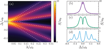
Fig. 4: (a) In color the emission spectrum,  , of the first site. Dashed white lines correspond to the eigenfrequencies of the system given by the imaginary part of eq. (7). (b)–(d)
  of the first site for different coupling strengths: (b)
  , (c)
, (c)  , (d)
, (d)  . In all figures N = 3,
  ,
,  and
and  .
.
Download figure:
Standard imageIn order to better understand these results we look at the spectrum ![$S(\Delta)=\sum_{l=1}^N \mathcal{S}^{(a)}_{1,k_l} \textrm{Re}[\langle \hat{a}^\dagger_1\hat{a}_{k_l}(\Delta)\rangle]$](https://content.cld.iop.org/journals/0295-5075/127/2/20001/revision1/epl19774ieqn157.gif) considering its components in the k-basis and for the different regimes. In the single-frequency regime we find
considering its components in the k-basis and for the different regimes. In the single-frequency regime we find
while in the two-frequency regime we find
The similitude between the expressions given in eqs. (19) and (20) and the ones obtained here, for the same regimes, is remarkable. In fact, in panels (b) to (d) of fig. 4 one can observe the same characteristic features of each regime: the interference windows in the single-frequency regime, and the expected Lorentzians in the two-frequency regime. These phenomena can be clearly identified in eqs. (33) and (34). In the single-frequency regime we always have  . Hence, from eq. (33), we clearly see that the spectrum is made of a Lorentzian dip with the smaller decay rate on top of a Lorentzian with the larger one. In fig. 4(b) all k-modes are in this regime, which explains the observed shape. This dip is also observed in panel (c) as
  is still below the critical value (EP). Thus, in eq. (33) we recognize a clear manifestation of the interference effect also found in the transmission spectrum: in the single-frequency regime two modes with the same frequency but different damping rate
  interfere destructively and inhibit (in the present case) thermal emission at a frequency in which the system is actually resonant.
In contrast, this interference effect is not present in the two-frequency regime. From eq. (34) we see that the spectrum is composed of different frequencies which, for large enough coupling strength, can be observed as well-defined resonance peaks in the spectrum (fig. 4(d)). These two different regimes have been observed in different physical systems, as, for instance, inhibited emission in a system of two coupled mechanical modes [32] (single-frequency regime) or the so-called parametric normal mode splitting in optomechanical systems [25,26] (two-frequency regime).
Concluding remarks
1D coupled open quantum systems with staggered losses display a rich dynamical scenario that emerges from the interplay between coherent and incoherent effects. By a detailed analysis of the dynamics for first and second moments, we disclosed qualitative different behavior as compared to what one would naively expect from the closed system, or from the uncoupled dissipative units. A major result of our analysis is the appearance of different regimes due to the progressive emergence of EPs, both in first and second moments dynamical equations, for increasing interaction strength. Remarkably, we have shown that the existence of EPs can even cause the whole open system to oscillate at a single frequency, despite the presence of a finite coupling strength between the many units. This single frequency emission can be achieved also in the limit of long chains, as the contrast is bounded by the bare coupling strength. In the presence of an external driving force, our open system presents peculiar properties in its transmission spectrum, such as transmission windows arising from destructive interference effects. The present results could be generalized to include additional effects, for example in the presence of frequency mismatch between units [52] and/or non-local dissipation effects [46,53].
Acknowledgments
The authors acknowledge support from MINECO/AEI/FEDER through projects EPheQuCS FIS2016-78010-P, CSIC Research Platform PTI-001, the María de Maeztu Program for Units of Excellence in R&D (MDM-2017-0711), and funding from CAIB PhD and postdoctoral programs.
Footnotes
- (a)
Contribution to the Focus Issue The Physics of Quantum Engineering and Quantum Technologies edited by Roberta Gitro, J. Gonzalo Muga and Bart A. van Tiggelen.