

Abstract
We consider two atoms trapped in a one-dimensional harmonic-oscillator potential interacting through a contact interaction. We study the response of the system against a monopolar perturbation during the transition from the non-interacting to the strongly interacting Tonks-Girardeau regime, as the interaction is varied from zero to infinitely large repulsive values. The response of the system is then characterized by the moments of the dynamic structure function which are explicitly calculated from the dynamic structure function and by means of sum rules.
Export citation and abstract BibTeX RIS
Introduction
Recent experiments with few ultracold atoms trapped in harmonic potentials have opened the way to understand how many-body quantum correlations build in few-body systems [1–8]. Such systems, if further confined to a one-dimensional (1D) geometry, offer an appropriate playground to study the interplay between quantum correlations and statistics [9].
The simplest example is that of two particles trapped in a harmonic-oscillator (h.o.) potential. For the case of a contact interaction potential [10], which is realistic for most ultracold atomic systems [11], two noteworthy limits are well known. In the absence of interactions the two atoms populate the lowest-energy single-particle state, producing the minimal version of a Bose-Einstein condensate. In the infinite interaction limit the two bosons resemble in many ways two spinless non-interacting fermions, producing the so-called Tonks-Girardeau (TG) limit [12]. The structure of the two-body system in the two limits is completely different [13], reflecting the nature of the correlations between the atoms [14–17].
One way to probe the correlations in a system is by studying its collective excitations. As discussed in ref. [18], the response to the monopolar operator is sensitive to the different regimes of the one dimensional bosonic gas. This is in contrast with the response to the dipolar operator, which excites the center-of-mass Kohn mode, which only depends on the trapping frequency, and thus provides no information about the internal correlations in the system. This has been one of the main experimental techniques used to discern between the different correlation regimes of ultracold bosonic gases. For instance, the mean-field Thomas-Fermi regime was achieved in the experiment of ref. [19] with 87Rb atoms exciting the breathing mode by modulating the optical lattice, i.e., changing the trapping potential, which is, in turn, equivalent to probing the system with the monopolar operator. The strongly correlated TG regime was explored later on in ref. [20] with Cs atoms. There, they used two different techniques to excite the breathing mode. In the mean-field regime they performed a sudden quench of the interaction strength, which was accurately controlled through a Feshbach resonance. In contrast, in the TG regime they used the monopolar operator, which in this case corresponded to an adiabatic compression of the cloud followed by a sudden removal of this extra trapping. A similar approach was followed in ref. [21], where the breathing mode was again excited by a sudden quench of the external harmonic trap. In all cases, the dipolar mode is measured by simply displacing the cloud and letting it oscillate in the trap.
In the two-boson system the situation is simpler. Even though the inner structure of the ground state is very different, the breathing mode of the trapped system has the same excitation energy of  for both the non-interacting and infinitely interacting limits, being ω the trap frequency [18]. This mode has actually two contributions. The first arises from the excitation of the center-of-mass mode. This contribution remains unchanged as we increase the atom-atom interaction and solely depends on the trapping potential. The second contribution is more intricate and corresponds to the first excited mode of the relative motion coupled to the ground state by the monopolar operator. The excitation energy of this mode changes as we vary the interaction strength. Starting at
  in the non-interacting case, it decreases as the atom-atom interaction strength is increased until it reaches a minimum. This increase of the interaction also builds up strong correlations between the two atoms. Past the minimum, the excitation energy increases with the interaction towards its limiting value of
  , i.e., the same value as the non-interacting case. This reentrant behavior of the breathing mode was discussed in ref. [22] and was in agreement with the Innsbruck experiment [20].
Several theoretical works have explored how the excitation energies can be extracted from the dynamical evolution of the system after a sudden quench in the trapping frequency. For instance, in refs. [23,24] the excitation energies were obtained from the Fourier analysis of the beating in the system after the quench. In their work, they used a multilayer multiconfiguration time-dependent Hartree method for bosons, which allows them to compute the dynamics for up to 5 particles. Direct diagonalization methods were used in ref. [25], where the breathing mode was studied in a Bose-Hubbard chain with an external trapping potential. There, the continuum was studied as a limiting case of the Hubbard model. A different approach was pursued in ref. [22]. There, quantum Monte Carlo calculations were performed for systems of up to N = 25 atoms. The method utilized was to determine the average excitation energy by means of sum rules [18,26,27], i.e., by computing the expectation value of certain operators in the ground state of the system.
In the present work we compute the dynamic structure function (DSF) by means of direct integration and sum rules, and study the response of the system associated to a monopolar excitation as we vary the atom-atom interaction, which is taken always repulsive. The article is organized in the following way. First, we describe the two-particle Hamiltonian. Next, we present the dynamic structure function computed at several interaction strengths. After that, we give explicit expressions for the sum rules applied to our system. Finally, we provide a summary and the main conclusions of our work.
Hamiltonian
The Hamiltonian for two bosons trapped in a one-dimensional h.o. and interacting through a contact potential reads

Here, we can define the center of mass (c.m.) and relative coordinates as  and
and  , respectively. Then, the Hamiltonian splits into two pieces,
  , which, written in the oscillator units of the original Hamiltonian, read

Note that, since the Hamiltonian splits into two commuting ones, the wave functions associated to the c.m. motion and the relative motion factorize,

Moreover, the full spectrum can be obtained as

where  is the spectrum of the c.m. h.o. Hamiltonian,
  , with k being the number of quanta associated to the c.m. motion, and
  is the spectrum of the relative motion Hamiltonian,
  , obtained via exact diagonalization. Recall that
  are upper bounds of the corresponding exact solutions since the diagonalization is performed on a truncated space.
In fig. 1 we depict the lowest part of the spectrum as a function of the atom-atom interaction constant, g. It can be readily seen how the eigenvalues evolve from the non-interacting bosonic system  to those of a free fermionic system
  . For instance, at g = 0, the ground state of H is non-degenerate and it is built with both atoms in the ground state of the h.o. single-particle Hamiltonian or as the product of the ground states of
  and
and  . Evidently, both descriptions provide the same energy, E = 1. However, in the
  limit, the ground state is the absolute value of the Slater determinant built with one atom in the ground state and the other in the first excited state of the h.o. single-particle Hamiltonian. Therefore, in this limit the ground-state energy (2 in h.o. units) is the sum of
  (ground state) and
  (first excited state) single-particle energies, and the contribution of the contact interaction is zero. Additionally, when one does the decomposition in
  and
and  , the ground state in the
  limit is achieved by taking the c.m. in the ground state (
 ), i.e., energy
  , and taking the relative wave function to be the absolute value of the first excited state, with energy
  , resulting in E = 2, as expected.
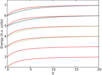
Fig. 1: Lowest-energy levels of the spectrum for the two-bosons system (see eq. (4)), for a range of interaction strength ![$g=[0,20]$](https://content.cld.iop.org/journals/0295-5075/127/5/56001/revision1/epl19834ieqn25.gif) . Red solid, green dotted and blue dashed lines correspond to c.m. excitations of the ground, first and second excited state of
. Red solid, green dotted and blue dashed lines correspond to c.m. excitations of the ground, first and second excited state of  .
.
Download figure:
Standard imageThe first excited state of the system, i.e.,  , corresponds to the first excitation of
  , with a constant excitation energy
  independent of g, and to the ground state of
  , with energy
  . In particular, all the excited states build with the corresponding c.m. excited state and the relative ground state result in a set of parallel curves, as depicted in red in fig. 1.
In the second excited state, i.e.,  , two states are found: one corresponds to two quanta of excitation of the c.m. combined with the ground state of
  (red line in fig. 1); the other one corresponds to the c.m. in the ground state and the relative motion in the first excited state of positive parity of Hr (green line in fig. 1). The two lines coincide at g = 0, where the energy level has degeneracy 2. Then, as g increases, the degeneracy is broken and the energy of the first excited state of the relative motion is always below the energy of the state with two quanta of excitation of the c.m. At
  the two states become again degenerated with total energy 4.
The transition from the BEC regime to the TG regime as the interaction strength is increased is shown in fig. 2. There, we report the total ground-state energy (red line) decomposed in kinetic energy  (blue line), harmonic oscillator potential energy
  (black line), and interaction energy
  (green line). We observe that
  increases monotonically from
  up to
up to  , while the kinetic energy starts at
  and goes through a minimum before growing up to
 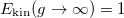 . Notice that both
  and
and  contain a constant contribution of the c.m. equal to 1/4. We also observe how the interaction energy increases with g until it reaches a maximum around
  . For
. For  the behavior changes and, despite the increasing atom-atom interaction strength, the interaction energy decreases monotonically as
  . Notice that, when
  , the exact wave function for the relative motion, built as
  (see eq. (3)), does not feel the contact interaction. This is a clear consequence of the formation of correlations in the system, which avoids the contact of the two bosons.

Fig. 2: Different contributors to the ground-state energy:  ,
,  and
and  , as functions of the interaction strength g. The total ground-state energy is shown in red,
  in blue,
  in black and
  in green (see legend).
Download figure:
Standard imageIn order to understand the behaviour of the different energy contributions for small g, we can combine a first-order perturbation theory estimate with the virial theorem. The virial relation,  , allows one to write

Therefore, we conclude that  for any value of g. Note that the equality only holds for g = 0 and
  . The correction to the energy is provided by the expectation value
  , where
  is the ground state of
  . Therefore,
  increases linearly with g. Using the previous relations for
  and
and  ,
,


These expressions agree well with the low-g regime depicted in fig. 2.
Dynamic structure function
The dynamic structure function encodes the response of our system to an external perturbation. Here we consider the case of a monopolar excitation. For a system with an arbitrary number of particles, N, the breathing mode can be excited by the one-body operator  . Its associated DSF reads

where  runs over the excited states,
  , and
, and  is the ground state. Thus, SF(E) can be explicitly computed with the eigenenergies and eigenfunctions of our system. In our numerical results, we truncate the infinite series to a finite number, D, which is the dimension of the truncated space of the diagonalization. In fig. 3 we depict the strengths of the DSF,
  , computed with N = 2 for four different values of g as a function of their excitation energy,
  . For g = 0 and g → ∞, SF(E) can be computed analytically. Notice that the excitation operator
  can be split into two pieces, one corresponding to the c.m. and the other to the relative motion, which in the case N = 2 reads
  .
.
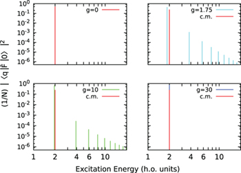
Fig. 3: Strengths of the dynamic structure function computed for a system composed by 2 bosons, with a delta contact potential. The value is calculated for g = 0, 1.75, 10, 30.
Download figure:
Standard imageFor g = 0 the two contributions excite two different states, both at the same excitation energy  , being
  the strength of the c.m. excitation and
  the one of the relative motion. The c.m. excitation generates only a peak at
  with strength
  , independently of the value of g. On the other hand, the internal excitations connected to the monopolar operator are distributed over several excited states, and the one accumulating most of the strength is known as the breathing mode. The strength of this peak grows monotonously from
  to
to  as g increases from 0 to infinity. This implies that, although both excitations, i.e., c.m. and breathing mode, have exactly the same energy, it is more likely to excite the breathing mode in the TG limit than in the BEC limit. Also, its excitation energy decreases for increasing values of g up to
  . Then, in the g → ∞ limit, it reaches again the excitation energy with value
  . This reentrant behaviour of the monopolar excitation is also reported in ref. [22]. In fig. 4 we report the strength of the breathing mode as a function of g, and the strength of the next three excited states of the relative motion. The strength of the breathing mode turns out to be an increasing function of g. This behaviour will be relevant to understand the evolution of the energy weighted sum rules of SF(E). In all the other cases, the strength is zero for g = 0 and increases with g up to a maximum, located around
  , to decrease again to zero as g → ∞. This maximum decreases when the excitation energy increases. Apparently, this dependence is very much correlated to the dependence of the interaction energy with g (see fig. 2).
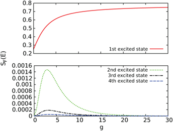
Fig. 4: Strength of the breathing mode (upper panel) and the next three higher relative states excited by the operator  (lower panel) as a function of the interaction strength g. They contain the factor
  .
.
Download figure:
Standard imageThe reentrant behavior presented by the excitation energy of the breathing mode also affects all the excited states of the relative motion. As shown in fig. 5 for several excited states, the reentrance energy, defined as  , is zero by definition at g = 0, whereas for increasing values of g it goes through a minimum to increase again asymptotically to zero when g → ∞. This reentrant behaviour is more pronounced for higher excited states. The maximum reentrance slightly shifts to higher values of g for higher excited states. Again, there seems to exist a correlation between the interaction energy and the reentrance energy as a function of g.
Fig. 5: Reentrance energy,  as a function of g for several excited states of Hr.
Download figure:
Standard imageSum rules
Computing the structure function explicitly becomes difficult for more than two particles. In particular, a naive second quantization scheme using the one-particle modes of the h.o. as single-particle states runs into difficulties as it mixes the c.m. with the relative motion in a non-trivial way [23]. A theoretical way to circumvent this problem would be to consider the excitation operator,  , as in [22]. An alternative method to characterize the dynamic structure function, SF(E), is by calculating its momenta Mn,

Note also that the momenta n and n + 2 provide estimates for the monopolar excitation energy. Assuming the structure function is concentrated around a single excitation energy,  , then we have
  for all n. The simplest one would be
  .
.
By means of sum rules, it is possible to compute several Mn without any explicit knowledge of all the eigenvalues and eigenvectors of the many-body system (see [26] and references therein). The sum rules below are derived in full generality, independently of the number of particles of the many-body system and, thus, they are particularly useful combined with Monte Carlo techniques which are able to describe the ground state [22].
 sum rule

To obtain the  sum rule we build a new Hamiltonian
  and consider the new term as a perturbation modulated by the parameter λ. The expansion up to second order of the ground-state energy,
  (eigenenergy of
  ) reads

where  and Eq are eigenstates and eigenvalues of the unperturbed Hamiltonian, respectively. Therefore,
  can be written as

Using also perturbation theory, we have an alternative expression for  ,
,

where  is the ground state of the perturbed Hamiltonian
  . For the present monopole operator,

where  is the single-particle ground-state density, with
  .
.
M1 sum rule
The M1 sum rule can be written as,

with  and
and  is the total harmonic potential energy. In ref. [22] the monopolar excitation energy is estimated by means of
  with
with  obtained from eq. (12).
M3 sum rule
Assuming that  is Hermitian, M3 can be calculated as

Alternatively, it can also be calculated as

where

M3 can then be computed as

Behaviour and asymptotic values of the sum rules
In fig. 6, M3, M1, and  are reported as functions of g. They have been calculated by explicitly integrating SF(E) and by using the previously presented formulas (see eqs. (11)–(18)). The agreement between both methods is excellent in the full range of g explored. All the sum rules are increasing functions of g and approach an asymptotic value for
  and, as expected, the convergence to the asymptotic values is faster for
  and slower for M3. However, all cases have almost reached convergence already for g = 30. This increasing character of the sum rules with g is mainly due to the increment of the strength of the breathing mode with g (see fig. 3). For all values of g, the peaks associated to the c.m. and to the breathing mode exhaust more than
  of the sum rules. The other peaks have a marginal influence, although they should be taken into account for the fulfillment of the sum rules (see, e.g., M3).
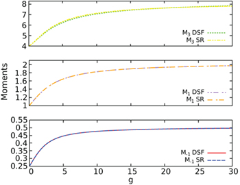
Fig. 6:  , M1 and M3 computed directly from SF(E) (DSF) and the sum rules (SR). When using SF(E) we have truncated the spectra by taking the first 10 energy levels.
Download figure:
Standard imageDue to the operator  the only excitation of the c.m. lies at an energy
  , above the ground state. The strength of this excitation (which contains the factor
  ) is
) is  and, therefore, the contribution to the different sum rules of the c.m. excitation is given by
  ,
,  , and
, and  . Recall that the contributions to the different sum rules of both the energy and the strength of the c.m. excitation are independent of g.
The non-interacting and the infinitely interacting limits are particularly amenable and allow one to compute the exact limiting values of the M1 and M3 sum rules. The two sum rules can be cast as functions of the average values of the kinetic and h.o. energies. The M1 and M3 sum rules for N particles read

where  and
and  are the expectation values of the total harmonic-oscillator potential energy and the total kinetic energy in the N-particle ground-state wave function, respectively.
For g = 0, the total, kinetic and harmonic potential energies are  ,
,  , and
, and  , respectively. Hence, for N = 2,
  and
and  , and the estimate of the monopolar excitation energy characterizing the dynamic structure function SF(E) is
  .
.
To evaluate the sum rules in the limit  we rely on the Bose-Fermi mapping. In the case of N particles they occupy the first N lowest single-particle energy levels of the h.o. potential so that

while  , and
, and  . Consequently,

which for N = 2 results in  and
and  . Then, the monopolar excitation energy calculated with M3 and M1 is, in this case,
  , which is the same as in the non-interacting case.
As the important peaks of SF(E), i.e., c.m. and breathing mode, are rather close to each other, one expects the estimate of the energy through the sum rules to be rather accurate. In fig. 7 we compare the monopolar excitation energies estimated by means of the sum rules with the values of the excitation energy,  (see eq. (4)). Notice that in all cases
  [26] for any value of g and both are larger than or equal to the minimum excitation energy defined by
  . First, we note that the two quantities obtained from
  and
and  do not produce the same estimate for the intrinsic monopolar excitation energy. This reflects the fact that the structure function contains two relevant excited states not located at the same energy, one from the c.m. and the second from the breathing mode. The difference between the two estimates provided by the sum rules increases with g and is larger for the value of g that maximizes the interaction energy. For this value of g the difference in energy between the c.m. excitation and the energy of the breathing mode is also maximal. Then, when g increases further and the breathing mode gets closer again to the c.m. excitation, the estimates get closer and both reach asymptotically
  when
when  . Subtracting the contribution of the c.m. to the sum rules, which is equivalent to study only the intrinsic excitations (see fig. 8), there is only one dominant peak and the estimations from the sum rules get much closer to each other. The differences in this case should be assigned to higher intrinsic excitations.
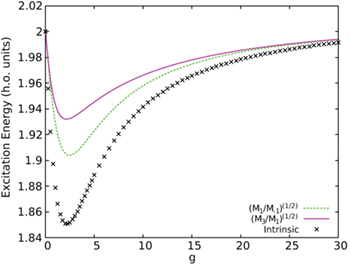
Fig. 7: Monopolar excitation energies obtained through  , M1 and M3, and first excitation energy from the spectra.
Download figure:
Standard image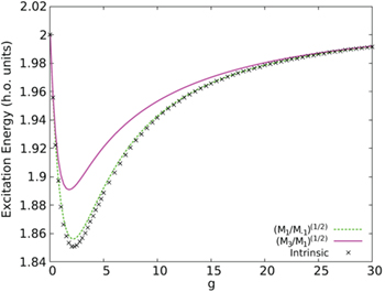
Fig. 8: Monopolar excitation energies obtained through  , M1 and M3, and the energy of the breathing mode. The contribution of the c.m. to the sum rules has been subtracted.
Download figure:
Standard imageSummary and conclusions
Unveiling the correlations present in many-body quantum systems is still a challenging task from both the experimental and theoretical point of view. With current experimental techniques in ultracold-atoms laboratories we can explore quantum correlations building in systems of very few number of atoms with control over trapping and interaction strengths.
In this case, we have considered a minimal setup of just two bosons in a one-dimensional harmonic trap. We varied the atom-atom interaction strength from zero to very large values, exploring the transition of the system from the BEC-like state to the TG-like one. The tool employed, which has been experimentally implemented in larger samples, is to study the response of the system to a monopolar excitation, e.g., quenching the trapping potential. In our case, we obtained the dynamic structure function of the system for different values of the interaction strength, explicitly computing its lower energy momenta. This tool also allowed us to benchmark the use of energy sum rules to compute the momenta of the structure function, a method employed, for instance, in quantum Monte Carlo approaches, finding a very good agreement between both methods. Then, we obtained estimates of the monopolar excitation energy, which is known to be directly related to the internal structure, and assessed the validity of simple estimates previously used in the literature, i.e.,  and
and  . Differences between both predictions reflect the fact that at least two peaks are always contributing to the structure function for any value of g. When the c.m. contribution is subtracted from the sum rules, the prediction of the excitation energy of the intrinsic breathing mode improves substantially. We expect to see important developments along these lines in near future experiments with few bosonic atoms.
Acknowledgments
The authors acknowledge useful discussions with Joan Martorell and Miguel Angel García March. We acknowledge financial support from the Spanish Ministerio de Economia y Competitividad Grant No. FIS2017-87534-P, and from Generalitat de Catalunya Grant No. 2017SGR533.