


Abstract
This paper carries out a cluster mean field analysis for spontaneous symmetry breaking in a two-lane totally asymmetric exclusion processes with an intersection. We find that the boundaries of the asymmetric phase are determined by differences of upstream segment densities and downstream segment flow rates of two lanes. The spontaneous symmetry breaking phenomenon exists when the interaction of particles is strong enough. The critical values, beyond which the phenomenon disappears, are identified through simulation and analysis, and they are in excellent agreement. The analytical results of the asymmetric phase boundaries are closer to simulation ones than those of simple mean field analysis. The analytical results of density profiles and the simulation ones are also in excellent agreement.
Export citation and abstract BibTeX RIS
Introduction
The transportation phenomenon is very common in our world, including microscopic objects such as ribosomes motion and protein synthesis, and macroscopic objects such as the vehicular traffic flow. In these phenomena, transport is often organized along linelike pathways, and interactions exist between entities [1]. The totally asymmetric simple exclusion process (TASEP) is considered to be the simplest model for studying various transport phenomena. In the model, particles move in one direction along a segment of consecutive sites but are subject to the principle of excluded volume. It was first introduced in 1968 to model mRNA translation by ribosomes [2]. Since then it is used as a predominant model to investigate stochastic dynamics along one-dimensional lattice [3], e.g., gel electrophoresis [4], polymer dynamics in dense media [5], diffusion through membrane channels [6], dynamics of motor proteins moving along rigid filaments [7,8] and dynamics of traffic flow [9–11]. Despite their simplicities, TASEPs can successfully explain some complex non-equilibrium phenomena such as boundary-induced phase transition [12–14], phase separation and condensation [15–19], shock formation [20–22] and so on.
In order to analyze more realistic situations that involves movement along multiple lanes, for instance, vehicle traffic, pedestrian flow and molecular motor motion, several studies investigated the multilane TASEP model [23–26]. In addition, in recent decades, the TASEP system with single species of particles was generalized to multispecies particles, exhibiting spontaneous symmetry breaking (SSB) when the microscopic symmetric dynamic rules lead to the existence of macroscopic asymmetric stationary-state properties for some sets of parameters [27–34].
Originally, the SSB was first observed in the single-lane exclusion process with two species of particles moving in the opposite directions, which is known as "bridge model" [27]. It is shown that two stationary phases with broken symmetry could exist for the same part of the parameter space, though the update rules are symmetric with respect to the two species. In the original model, particles of different species interact with each other at every site of the lane. Later, the study was extended to two-channel asymmetric exclusion processes with narrow entrances where particles move on two parallel lanes, two species of particles only interact at entrances [25]. The study was also extended to a new class of bridge model fed by junctions [35]. It is found that the local interaction strongly influences the macroscopic particle dynamics of the system. However, understanding of the nature of the SSB phenomenon is still an open question. It is known that the SSB is not observed in the single species system [26].
In molecular motor motion, molecular motors move along filaments, the filaments may be crossed with each other. When the molecular motors arrive at the intersection, they may go to each of the two filaments. In vehicle traffic, drivers usually know where the destination is. When they arrive at crossroads, they may change road if the pre-defined moving road is in congestion. Motivated by these phenomena, Yuan et al. have studied two-lane TASEP in which the two lanes intersect at a center site. In this model, the SSB phenomenon is also observed [23]. The model was analyzed using the simple mean field (SMF) approach in which correlation of sites is ignored. Four phases are identified in simulations, while only three phases excluding the asymmetric phase can be predicted in the analysis. The asymmetric phase cannot be analyzed. Later, Zhu et al. studied another TASEP on two intersected lanes, and the SSB phenomenon exists. Motivated by the fact that the simple mean field (SMF) fails to investigate the asymmetric phase, the cluster mean field (CMF) analysis was adopted. In the analysis, correlation of three sites (i.e., intersected site, two upstream sites next nearest to the intersected site) was considered. The boundaries of the asymmetric phase are determined by the difference of densities of two lanes [36]. However, the downstream sites next nearest to the intersected site were not considered in the analysis, and it is not known whether flow rates of two lanes have effect on the boundaries of the asymmetric phase.
In the present paper, we investigate the two-channel TASEP model with an intersection in ref. [23] by simulation and analysis. We focus on the SSB phenomenon. Through simulation, it is found that the region of the asymmetric phase changes gradually in the phase diagram with the change of parameter. Only when the interaction of particles is strong enough, the SSB phenomenon is observed. To analyze the change of the asymmetric phase quantitatively, we adopt the cluster mean field (CMF) approach in the analysis. The correlation of the intersected site and four sites next nearest to it are considered. We find that the boundaries of the asymmetric phase are determined by differences of densities and flow rates of the two lanes, and the simulation results and analytical results are in excellent agreement. The proposed system and the analysis help to better understand the non-equilibrium transport phenomena observed at macroscopic and microscopic level.
This paper is organized as follows. In the next section, we present a detailed description of the model. In the third section, we analyze the system using the cluster mean field and simple mean field approaches, and we compare the analytical results with simulation ones. We summarize and conclude in the forth section. We describe master equations used in the cluster mean filed analysis in the Supplementary Material Supplementarymaterial.pdf (SM).
Model
In this section, the update rules of the model are introduced. In the model, the system consists of two one-dimensional lanes with an intersection under the open boundary condition. Lane 1 is in the horizontal direction and lattices are numbered from 1 to L, while lane 2 is in the vertical direction and lattices are numbered from L+1 to 2L. The random update rule is adopted. At the entrance site, a particle is inserted with rate α provided the site is empty. At the exit site, a particle is removed by rate β. In the bulk (except for site C), a particle hops to the next site with rate 1 provided the target site is empty. The lanes are sketched in fig. 1.
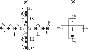
Fig. 1: (a) Sketch of the model. The arrows show allowed hopping and the crosses show prohibited hopping. Entrance rates at both lanes are equal to α and exit rates are equal to β. Filled circles indicate that the sites are occupied by particles. (b) The sketch of the five sites and effective injection rates and removal rates in the cluster mean field analysis of the model.
Download figure:
Standard imageIn the model, there are two types of particles which correspond to the vehicle traffic or molecular motor motion. Type 1 enters from site 1 and type 2 enters from site L+1. If site C is occupied by a particle of type 1(2), the particle moves to the site C3(C4) with rate 1 if site C3(C4) is empty independent of the status of site C4(C3), and the particle moves to the site C4(C3) with rate p if site C3(C4) is occupied and C4(C3) is empty. Here p controls the strength of the interaction at the intersected site. With decrease of p, the interaction of particles at the intersection increases.
Analytical and simulation results
The analytical and simulation results are discussed in this section. The phase diagram is shown in fig. 2. When p = 0, there exist three phases, i.e., symmetric LL phase, symmetric HL phase and asymmetric phase. In the symmetric LL phase, two lanes are both in low densities, see fig. 3(a). In the symmetric HL phase, the system is in the high-density upstream of the intersection site and in the low-density downstream of the site, see fig. 3(b). In the asymmetric phase, one lane is in high density, the other lane is in the HL phase, see fig. 3(c) and fig. 3(d). When  , the asymmetric phase exists, which is reported in ref. [23]. Through simulation, we find that the asymmetric phase shrinks with the increase of p. Moreover, a new symmetric HH phase appears, in which the two lanes are both in high densities. The symmetric HH phase expands with the increase of p. When p > pcr, the asymmetric phase disappears. In ref. [23], the theoretical boundaries were investigated by simple mean field analysis, in which the correlation of sites is ignored. It has been found that when the system is in the symmetric LL phase, the following conditions should be satisfied:

When

the system is in symmetric HH phase.
When

the system is in symmetric HL phase.
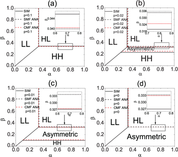
Fig. 2: The phase diagram of the model, obtained from simple mean field analysis (black dashed lines), cluster mean field analysis (red dashed lines) and Monte Carlo simulations (black solid lines). The parameter is (a)  , (b)
, (b)  , (c)
, (c)  , (d) p = 0.
Download figure:
Standard image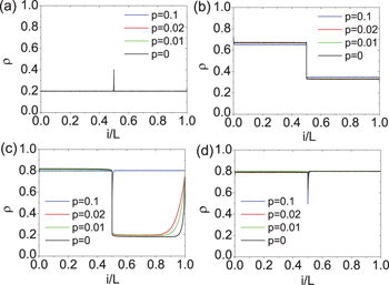
Fig. 3: The density profiles obtained from Monte Carlo simulations corresponding to different values of p. (a) The symmetric LL phase, with the parameters  ,
,  . (b) The symmetric HL phase, with the parameters
  ,
,  . (c) The HL phase (p = 0, 0.01, 0.02) and the HH phase (
 ) of one lane in the system, with the parameters
  ,
,  . (d) The HH phase of the other lane in the system, with the parameters
  ,
,  .
.
Download figure:
Standard imageFrom the analysis, we know that the asymmetric phase could not exist. This is because of the neglect of the correlation of sites. The simple mean field analysis predicts that there are three phases in the system, which is not in accordance with simulation results, see fig. 2(b) and fig. 2(c).
In the model, p represents the strength of the interaction at the intersection. With the increase of p, the interaction decreases, and the asymmetric phase is suppressed. Then the asymmetric phase exists only when p is small enough. The asymmetric phase exists when α is large and β is small. The appearance of the asymmetric phase can be qualitatively explained as follows. It is initially supposed that segments II and IV are empty, see fig. 1(a). When particles reach the exit sites of the two segments, the shock will form on the two segments and propagate upstream because the removal rate is smaller than the effective entrance rate in the two segments. One of the shock reaches site C first, which leads to the stable HD phase in the segment. On the other hand, a barrier is formed at site C, which leads to a significant decrease of the effective entrance rate in the other segment. Thus, LD phase instead of HD phase exists in the other segment. As a result, the system is found in the asymmetry phase with one lane in the HH phase and the other one in the HL phase.
In this paper, we carry out the analysis of the asymmetric phase using the cluster mean field approach in this model. The update of particle in the intersection site (site C) is related to the conditions of sites C3 and C4, the five sites (sites C, C1, C2, C3, C4) are considered in the analysis, see fig. 1(b).
Let  and
and  denote the effective injection rates into site i and m;
  and
and  denote the effective removal rates of particles from site k and n;
  denote the probability that site i in state
  , site j in state
  , site k in state
  , site m in state
  , site n in state
  , and
, and  ,
,  ,
,  ,
,  can only be 0 and 1 (0 means empty, 1 means occupied),
  can be 0, 1 and 2 (0 means empty, 1 means occupied by an eastbound particle, 2 means occupied by a northbound particle); J1 and J2 denote the flow rates of the upstream of the intersection site on the eastbound and northbound lanes; J3 and J4 denote the downstream flow rates on the eastbound and northbound lanes;
  and
and  denote the densities of sites i and m.
Now we can write the master equations of  . Take P00000 for example,

and the other equations are shown in the SM. In the stationary state, we obtain  . Therefore, we have 48 equations, but only 47 of them are independent ones. Due to the conservation of probability, we can obtain that

Furthermore,  and
and  are given by
In addition, by ignoring correlations, the relationship between  and J1,
  and J2 can be obtained:


J1 and J2 can also be expressed as


On the other hand, J3 and J4 can be calculated by


In the asymmetric phase, one lane is in high density (HD), the other lane is in the HL phase. Without loss of generality, we suppose that the eastbound lane is in the HD phase and the northbound lane is in the HL phase. Then J3 is determined by

Since the northbound lane is in the HL phase, which means that the upstream segment of the intersection site is in high density and the downstream segment is in low density. Thus J4 can also be calculated by

Now we have 58 unknowns, including 48 probabilities  ,
,  ,
,  ,
,  ,
,  ,
,  ,
,  , J1, J2, J3 and J4. We also have 58 equations, i.e., eqs. (4)–(15) and (A1)–(A46). We can solve the equations to obtain
  ,
,  , J1, J2, J3 and J4. We have plotted the differences between
  and
and  , J3 and J4 vs. β when p = 0, see fig. 4.
It can be seen that  and
and  are both positive in the range of
  . The differences decrease when β approaches
  .
.  and
and  when
when  . In the analysis of the asymmetric phase, we suppose that the eastbound lane is in the high density and the northbound lane is in the HL phase. It means that the density of the upstream of the intersection site of the northbound lane is larger than that of the eastbound lane, i.e.,
  . The flow rate of the downstream of the intersection site of the northbound lane is smaller than that of the eastbound lane, i.e.,
  [37,38]. Therefore, the asymmetric phase exists when
  , see fig. 4. The system is in symmetric HL phase when
  .
.
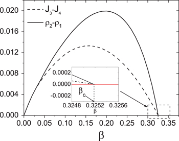
Fig. 4: Dependence of  (solid line) and
  (dashed line) on β in the range
  when p = 0, obtained from cluster mean field analysis.
Download figure:
Standard imageWhen p > 0, take  for example, the relations of
  ,
,  and β can also be obtained, see fig. 5.
  is also positive in the range
  . However, only when
  ,
,  is positive, and
  . It means that when
  ,
,  is satisfied but
  is not. Therefore, the asymmetric phase exists when
  . When
  , the system is in symmetric HH phase. It means that the bottom boundary of the asymmetric phase is determined by the difference of flow rates of the two lanes' downstream segments, and the top boundary boundary is determined by the difference of densities of the two lanes' upstream segments.
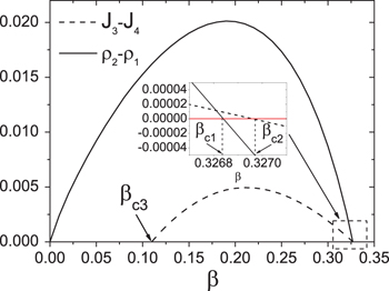
Fig. 5: Dependence of  (solid line) and
  (dashed line) on β in the range
  and
and  when
when  , obtained from cluster mean field analysis.
Download figure:
Standard imageActually, in the model of ref. [36] and when p = 0 in the present model, two particles of different species cannot change hopping directions. Then the flow rates of upstream and downstream segments of the same lanes are equal, i.e.,  and
and  are always satisfied. When
  ,
,  . The values of
  corresponding to the asymmetric phase boundaries determined by the difference of densities of upstream segments of the two lanes are identical to that determined by the difference of flow rates of downstream segments of the two lanes. However, when p > 0 in the present model, particles may change hopping directions at the intersection, then
  and
and  . When
  ,
,  may not be satisfied. The
  obtained from the differences of the densities and flow rates are not identical. From fig. 5 and fig. 6, we can see that
  and
and  . The differences of the densities of the upstream segments and flow rates of the downstream segments of two lanes together determine the boundaries of the asymmetric phase.

Fig. 6: Dependence of  (solid lines) and
  (dashed lines) on β with different value of p, obtained from cluster mean field analysis.
Download figure:
Standard imageWith the increase of p,  increases, see fig. 6. It means that the asymmetric phase shrinks and the symmetric HH phase expands when p increases. Through analysis, we find that when
  which is very close to the simulation value
  . When
  becomes equal to
  , the asymmetric phase disappears.
From the analysis, in the asymmetric phase,  , which means that the density of the upstream segment of the intersection site on the lane with HL phase is larger than that of the lane with HD phase. This is in accordance with the simulation, see fig. 7. In fig. 7, the densities obtained from simulation and analysis are in excellent agreement. Following the parameters presented in fig. 7, the values of flow rates of the downstream segment of the lane with HL phase and HD phase obtained from simulations are 0.151738, 0.164441, and the values obtained from analysis are 0.151459, 0.163657. The flow rates from simulation and analysis are also in excellent agreement.

Fig. 7: The density profiles obtained from Monte Carlo simulations (dashed lines) and cluster mean field analysis (solid lines). The black and red lines represent HD and HL phases. The parameters are  ,
,  and
and  .
.
Download figure:
Standard imageIn this model, when  , the asymmetric phase does not exist, and the boundary
  between the symmetric HH phase and the symmetric HL phase can also be calculated. In the symmetric HL phase, the two lanes are both in HL phase. The upstream segments of the intersection site on both lanes are in high density and the downstream segments on two lanes are in low density. Because of the symmetry,
  ,
,  ,
,  ,
,  ,
,  , therefore we have 53 unknowns, including 48 probabilities,
  ,
,  , J1(J2), J3(J4) and
  . We also have 53 equations, i.e., eqs. (4)–(6), (8), (10), (13), (15) and (A1)–(A46). We solve these equations, and the boundary is determined by

We also compare the analytical results with the Monte Carlo simulation ones in fig. 2(a) and fig. 8. In fig. 2(a), the cluster mean field analytical results are closer to the simulation ones than those of the simple mean field analysis. In fig. 8, the analytical results are in excellent agreement with the simulation ones.
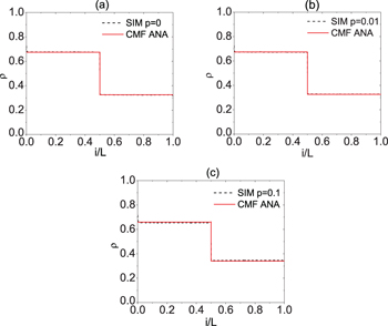
Fig. 8: The density profiles of the symmetric HL phase. The black dashed lines are obtained from Monte Carlo simulations. The red solid lines are obtained from the cluster mean field analysis. The parameters are  ,
,  and (a) p = 0, (b)
  , (c)
, (c)  .
.
Download figure:
Standard imageConclusion
To summarize, we have studied the model of the totally asymmetric simple exclusion process on two intersected lanes under open boundaries with random update. In the model, two types of particles move in two lanes. In the intersected site, a particle can change the moving lane with rate p. Extensive Monte Carlo simulations show that there are four phases (symmetric HH phase, symmetric HL phase, symmetric LL phase and asymmetric phase) in the system when  . When
  , the asymmetric phase disappears.
In the simple mean field analysis, correlation between sites is ignored. The analysis indicates that three phases (symmetric HH phase, symmetric HL phase, symmetric LL phase) exist in the system, and the asymmetric phase cannot be obtained. With the decrease of p, the interaction of particles at the intersection increases, and the correlation becomes stronger. The simple mean field approach cannot be used in the analysis. Motivated by this, we have carried out the cluster mean field analysis for the model. Five sites including the intersection site are considered in the analysis because the motion of the particle in the intersection site is related to the nearest-neighbor two sites in every lane.
In the cluster mean field analysis, the analytical boundaries and density profiles are obtained. For the analytical boundaries, the cluster mean field analytical results of boundaries of the asymmetric phase are closer to the simulation ones than those of the simple mean field analysis, this is because the correlation of sites is considered. The top boundary of the asymmetric phase is determined by the difference of densities of upstream segments of the two lanes, and the bottom boundary of the asymmetric phase is determined by the difference of the flow rates of downstream segments of the two lanes. With increase of p, the analysis indicates that the asymmetric phase shrinks. When  , the asymmetric phase disappears. It is very close to the simulation value of
  . For the density profiles, when the system is in the asymmetric phase, the cluster mean field analysis indicates that the density of the upstream segment of the intersection in the lane with HL phase is larger than that of the lane with HD phase, this is in accordance with the simulation. When the system is in the asymmetric phase and in the symmetric HL phase, the cluster mean field analytical results of density profiles and simulation ones are both in excellent agreement.
Acknowledgments
This work is supported by the National Natural Science Foundation of China (Grant Nos. 11802003, 71621001, 11672289 and 71671058).