

Abstract
After the Bak-Tang-Wisenfeld seminal work on self-organized criticality (SOC), the following claim appeared by other workers in the 1990s: Earthquakes (EQs) cannot be predicted, since the Earth is in a state of SOC and hence any small earthquake has some probability of cascading into a large event. Here, we discuss that such claims do not stand in the light of natural time analysis, which was shown at the beginning of the 2000s to extract the maximum information possible from complex systems time series. A useful quantity to identify the approach of a dynamical system to criticality is the variance  of natural time χ, which becomes equal to 0.070 at the critical state for a variety of dynamical systems. This also holds for experimental results of critical phenomena such as growth of ricepiles, seismic electric signals activities, and the subsequent seismicity before the associated main shock. Another useful quantity is the change
  of the dynamic entropy
  under time reversal, which is minimized before a large avalanche upon analyzing the Olami-Feder-Christensen model for EQs in natural time. Such a minimum actually occurred on 22 December 2010, well before the M9 Tohoku EQ in Japan on 11 March 2011, being accompanied by increases of both the complexity measure of the
  fluctuations and the variability of the order parameter of seismicity (which was minimized two weeks later). These increases conform to the seminal work on phase transitions by Lifshitz and Slyozov and independently by Wagner as well as to more recent work by Penrose et al. In addition, the evolution of the complexity measure of the
  fluctuations reveals a reliable estimation of the occurrence time of this M9 EQ.
Export citation and abstract BibTeX RIS
Introduction
In geoscience, considerable interest on power law distributions, or more correctly, power-law–like probability distributions [1], arose in the 1980s due to the appealing work of Mandelbrot on fractals [2], which drew attention to the distribution of sizes of various geological objects and structures, like lakes, faults, fault gouges, oil reservoirs, sedimentary layers, etc. [3]. In the 1990s, after the seminal work of Bak and coworkers [4,5] on self-organized criticality (SOC), the above interest was reinforced in particular regarding catastrophic geophysical phenomena that can be considered to happen in terms of "avalanches" (events which suddenly release energy slowly accumulated in the system).
The fact that avalanches were taken [4] as uncorrelated in the SOC archetype, the sandpile, has been used as an argument that it is not possible to predict the occurrence of large avalanches such as earthquakes (EQs) (relevant claims are cited in [6,7]) since at any moment any small avalanche can eventually cascade to a large event.
To shed more light towards answering the aforementioned question on EQs predictability, we employed natural time analysis, which has been shown since the beginning of the 2000s [8,9] to unveil hidden properties in complex time series. Natural time has been used as basis for the development by Turcotte, Rundle and coworkers [10,11] of a new method for a quantitative evaluation of the current level of seismic risk. Here, after describing in short the background of this analysis in the next section, we explain the results of its application to the following cases: First, time series of avalanches in laboratory measurements on SOC systems. Second, a pronounced minimum of the entropy change of seismicity under time reversal appeared [12] before the super-giant M9 Tohoku EQ in Japan on 11 March 2011. Third, the evolution of the fluctuations of the latter entropy change is of paramount importance for the identification of the occurrence time of this EQ [13].
Natural time analysis: background
For a time series comprising N events, we define an index for the occurrence of the k-th event by  , which we term natural time [8,9,14]. In doing so, we ignore the time intervals between consecutive events, but preserve their order and energy Qk
. We, then, study the pairs
, which we term natural time [8,9,14]. In doing so, we ignore the time intervals between consecutive events, but preserve their order and energy Qk
. We, then, study the pairs  , by using the normalized power spectrum
  defined by
  , where ω stands for the angular natural frequency and
  is the normalized energy for the k-th event.
In the time-series analysis using natural time, the behavior of  at ω close to zero is studied for capturing the dynamic evolution, because all the moments of the distribution of the pk
can be estimated from
at ω close to zero is studied for capturing the dynamic evolution, because all the moments of the distribution of the pk
can be estimated from  at
at  (see ref. [15], p. 499). For this purpose, a quantity
  is defined from the Taylor expansion
  , where

We found that this quantity, the variance of natural time  , is a key parameter for the distribution of energy within the natural time interval
 ![$(0,1]$](https://content.cld.iop.org/journals/0295-5075/132/2/29001/revision2/epl20386ieqn17.gif) . Note that
. Note that  is "rescaled" as natural time changes to
  together with rescaling
  upon the occurrence of any additional event. It has been demonstrated that this analysis enables recognition of the dynamic complex system entering the critical stage [8,9,14,16]. This occurs when
  converges to 0.070. Originally the condition

for the approach to criticality was theoretically derived [8,9] for the seismic electric signals (SES) activities, which are series of transient low-frequency ( ) electric signals observed before EQs [17] with lead time from a few weeks to around
  months [14] (generated by a second-order phase transition [14,17]). The experimental data showed that
  of SES activities in Greece and Japan attain the value 0.070 [8,9,14,18]. The condition
  holds for other time series, including several dynamical models [14] and seismicity preceding mainshocks [14,18–20].
The entropy S in natural time (which is a dynamic entropy and not a static one, e.g., Shannon entropy [21–23]) defined in ref. [24] is

where  denotes the average value of
  weighted by pk
, i.e.,
weighted by pk
, i.e.,  and
and  . The entropy obtained by eq. (3) upon considering [14,25] the time reversal
  , i.e.,
  , is labelled by
  :
:

 is different from S, thus there exists a change
  in natural time under time reversal. Hence, S does satisfy the condition to be time-reversal asymmetric [14,23,25]. It constitutes the basis for the introduction of proper complexity measures to distinguish, in the analysis of electrocardiograms for example [23], sudden-cardiac-death (SCD) individuals from healthy ones [21–23], as well as to identify in SCD when ventricular fibrillation starts.
The quantity  is of key importance to identify also when a system approaches a dynamic phase transition. Its calculation is carried out by means of a window of length i (
 of successive events), sliding each time by one event, through the whole time series. The entropies S and
  , and therefrom their difference
  , are calculated each time. Thus, we form a new time series comprising successive
  values.
Computing the standard deviation  of the time series of
  , the complexity measure
  , which is particularly very useful for the analysis of EQ catalogues, is defined by [14,26]

where the denominator stands for the standard deviation  of the time series of
  of
of  events. Note that the selection of a different scale in the denominator, e.g., i = 50 or 200 events, instead of i = 100 events, would change of course the numerical values obtained but the whole behavior and physical picture of the results concerning the time evolution of
  would remain the same [13].
  quantifies how the statistics of
  time series varies upon changing the scale from 100 to another scale i, and is of profound importance to study the dynamical evolution of a complex system (see p. 159 of ref. [14]).
Natural time analysis of laboratory measurements
In experiments on a three-dimensional pile of long-grained rice it was found [27] that there is an additional factor for obtaining SOC behavior in a granular pile: the boundary condition of the system. If the foot of the pile rests on a flat surface, power-law–distributed avalanches over almost four orders of magnitude are observed. However, if the foot of the pile is at the edge of the surface on which the pile rests such that grains can fall off the edge, we observe quasiperiodic system-spanning avalanches, in addition to the power-law–distributed small- and medium-sized avalanches. Since this boundary condition is similar to the one used in some of the sandpile experiments, these findings may help to explain why the archetype of SOC, the sandpile, was found to have power-law–distributed avalanches in some experiments, while in other experiments quasiperiodic system-spanning avalanches were found.
Since avalanches in sandpiles as the most commonly used paradigm for SOC behavior have been put under question, Denisov et al. [28] investigated experimentally whether SOC occurs in granular piles composed of different grains, namely, rice, lentils, quinoa, and mung beans. These four grains were selected to have different aspect ratios, from oblong to oblate. It was found that only rice (with rice grains having a very high aspect ratio) exhibits a truly SOC behavior. Hence, natural time analysis was applied to the experimental data of the well-controlled experiments performed in refs. [29,30] on three-dimensional (3D) ricepiles. The relevant results reviewed in ref. [14], led to the following average values (standard deviation) of the quantities  , S and
  when the system enters the critical state:
  , hence being in accordance with eq. (2),
  and
and  (obeying the additional conditions S < Su
and
(obeying the additional conditions S < Su
and  for criticality [20], where Su
stands for the entropy of a uniform distribution [14]). Natural time analysis was also applied to time series of avalanches from other laboratory systems exhibiting SOC, e.g., magnetic flux penetration in thin films of YBa2Cu3O
for criticality [20], where Su
stands for the entropy of a uniform distribution [14]). Natural time analysis was also applied to time series of avalanches from other laboratory systems exhibiting SOC, e.g., magnetic flux penetration in thin films of YBa2Cu3O [31].
[31].
Natural time analysis reveals that the entropy change under time reversal is minimised before a major earthquake
Upon analyzing the Olami-Feder-Christensen (OFC) model for EQs in natural time, a non-zero change  of the entropy in natural time upon time reversal is identified [14,32], which reveals a breaking of the time symmetry, thus reflecting the predictability in the OFC model. This model is probably [7] the most studied non-conservative, supposedly, SOC model and has been a mainstream tool to study the SOC behavior of earthquake dynamics, because it can reproduce many critical features of real-world earthquakes, see ref. [33] and references therein. In particular, in the OFC model, it was found (see fig. 8.12, p. 361 of ref. [14]) that
  exhibits a minimum [14] (or maximum if we define [32]
  , instead of
  ) before large avalanches.
In view of this finding, a natural time analysis of all earthquakes in Japan above a magnitude (M) threshold from 1 January 1984 until the occurrence of the super giant M9 Tohoku earthquake on 11 March 2011 was made [12] as follows: The Japan Meteorological Agency (JMA) seismic catalogue was used (e.g., see [34,35]). The energy of EQs was obtained from the JMA magnitude M after converting [36] to the moment magnitude Mw
[37]. Setting a threshold  to assure data completeness, there exist 47204 EQs in the concerned period of about 326 months in the entire Japanese region, i.e.,
  . Thus, we have on average
  EQs per month.
The time evolution of  was studied [12] for a number of scales i of the seismicity by selecting proper values of i on the basis of the fact that natural time analysis demonstrated the following interconnection between SES activities and seismicity [38]: The fluctuations, or the variability β [14,34], of the order parameter
  of seismicity (for the definition of β see eq. (6) that will be discussed later) exhibit a minimum labeled
  when we observe the initiation of a SES activity whose lead time ranges, as already mentioned, from a few weeks up to around
  months [14]. A SES activity, exhibiting critical behavior [9,24], is observed during a period in which long-range correlations prevail between EQ magnitudes [39]. On the other hand, well before the initiation of the SES activity, and hence before
  , a different stage appeared in which the temporal correlations between EQ magnitudes exhibited an anticorrelated behavior [39]. Hence, there exists a significant change in the temporal correlations between EQ magnitudes when comparing the two stages that correspond to the periods before and just after the initiation of a SES activity. Since this change was likely to be captured by the time evolution of
  , the study of
  should start from the scale of
  events, which is approximately the number of seismic events
  occurring on average during a period around the maximum lead time of SES activities.
A careful inspection of the plots of  values vs. the conventional time for the scales
  ,
,  ,
,  ,
,  ,
,  ,
,  and
and  seismic events reveals [12] the following common feature: At shorter scales, i.e., from
  to
to  events, a number of local minima appear, but leaving aside all these changes we find that at longer scales, i.e.,
  ,
,  and
and  events (see fig. 1) a pronounced minimum is observed on 22 December 2010 (upon the occurrence of a M7.8 EQ in southern Japan at
  N
N  E) almost two and a half months before the M9 Tohoku EQ. This minimum
  of
of  of seismicity in the entire Japanese region under time reversal is statistically significant because the probability to observe by chance such a deep (or even deeper) minimum was estimated [12] to be close to 3%. In addition
  can be considered as a precursor to the M9 Tohoku EQ, since it has a very small probability (<1%) to occur by chance as shown in ref. [40] when employing the recently introduced method of event coincidence analysis [41,42]. Furthermore, note that the robustness of the appearance of
  on 22 December 2010 was also investigated [12] upon changing the EQ depth.

Fig. 1: Plot of  values vs. the conventional time. Panels (a), (b) and (c) correspond to the scales
  ,
,  and
and  events, respectively, when analyzing all EQs with
  within the entire Japanese region
  from 1 January 1984 until the occurrence of the M9 Tohoku EQ on 11 March 2011. Panels (d), (e) and (f) correspond to excerpts of panels (a), (b) and (c), respectively during the
  month period from 1 October 2010 until the M9 Tohoku EQ occurrence on 11 March 2011. The higher two vertical lines ending at circles depict the magnitude (
 ) EQs read in the right scale that correspond to the M7.8 EQ on 22 December 2010 and the M9 Tohoku EQ on 11 March 2011. For additional scales see figs. 2–4 in ref. [12].
Download figure:
Standard imageIn short, upon analyzing in natural time the seismicity in Japan from 1 January 1984 until the occurrence of the M9 Tohoku supergiant EQ on 11 March 2011, we find that for longer scales, i.e., i > 3500 events, the minimum of  is observed on 22 December 2010. This is consistent with the aforementioned finding in the OFC model.
In addition, studying the complexity measure  vs. i at the scales
  , 3000 and 4000 events, Varotsos et al. [43] found an evident increase
  on 22 December 2010 upon the occurrence of the aforementioned M7.8 EQ obeying a scaling behavior of the form
  , where the exponent c is independent of i with a value very close to
  , while the pre-factors A are proportional to i and t0 is approximately 0.2 days after the M7.8 EQ occurrence. This behavior conforms to the seminal work by Lifshitz and Slyozov [44] and independently by Wagner [45] on phase transitions which shows that the time growth of the characteristic size of the minority phase droplets grows with time as
  . Furthermore, the quantity

defined [14] as the variability of the order parameter  of seismicity, the time evolution of which can be pursued by sliding the excerpt of length i through the EQ catalogue and computing the average
  and the standard deviation
  of the thus-obtained ensemble of
 ![$[(i-4) (i-5)] / 2 \kappa_1$](https://content.cld.iop.org/journals/0295-5075/132/2/29001/revision2/epl20386ieqn109.gif) values [35], reveals the following behavior [40]: Upon increasing i, it is observed (see figs. 2(B) and 4(E) of ref. [34]) that the increase
values [35], reveals the following behavior [40]: Upon increasing i, it is observed (see figs. 2(B) and 4(E) of ref. [34]) that the increase  of the
  fluctuation, upon the occurrence of the above M7.8 EQ on 22 December 2010, becomes distinctly larger, which does not happen (see figs. 4(A)–4(D) of ref. [40]) for the increases of the β fluctuations upon the occurrences of all other shallow EQs in Japan of magnitude 7.6 or larger during the period from 1 January 1984 to the time of the M9 Tohoku EQ. Such a behavior that obeys the inter-relation
  (see figs. 2(g) and (h) of ref. [40]) has a functional form strikingly reminiscent of the one discussed by Penrose et al. [46] in computer simulations of phase separation kinetics using the ideas of Lifshitz and Slyozov [44], see their eq. 33 which is also due to Lifshitz and Slyozov (cf. remarkably, after the publication of ref. [40], an inter-relation of similar form, i.e.,
  was also observed upon the occurrence of a M6.4 EQ almost 34 h before the M7.1 Ridgecrest EQ in California that struck on 6 July 2019 at 03:20 UTC). Hence, the β fluctuation on 22 December 2010 accompanying the minimum
  is unique. By employing the event coincidence analysis [41], which considers a time lag τ and a window
  between the precursor and the event to be predicted, the profound statistical significance of this unique result has been further assured as follows [40]: Assuming the M9 Tohoku EQ as the event to be predicted, the probability (p-value) that the increased fluctuation on 22 December 2010 is a chancy precursor with a lag τ and a window
  , i.e., the EQ occurs within the time period from τ to
  days later, was found to be very small, i.e., from
  to 0.01% when
  varies from 78 days to 1 day, respectively.
Natural time analysis: estimation of the occurrence time of an impending major earthquake by means of the fluctuations of the entropy change under time reversal
As mentioned in the second section, the key point for the estimation of the occurrence time of an impending mainshock is the attainment of the condition  for seismicity when analyzing in natural time the consecutive EQs subsequent to the SES activity initiation. Even without using this condition, however, it has been recently shown [13] that the occurrence time of an impending mainshock can be identified by studying the evolution of the complexity measure
  of seismicity explained below taking as an example the M9 Tohoku EQ in Japan on 11 March 2011.
Concerning the minimum of  on 22 December 2010, upon the occurrence of the aforementioned M7.8 EQ, a significant change in the temporal correlations of the EQ magnitude time series in Japan has been observed, as mentioned, as follows: The magnitude time series before major EQs have been investigated in ref. [39] in the entire Japanese region (
 ) during the period from 1 January 1984 until the M9 Tohoku EQ occurrence by employing the detrended fluctuation analysis (DFA) [47]. For each target EQ, the magnitudes of i = 300 consecutive events before the target have been analyzed [39] and a DFA exponent α was therefrom deduced, where
  means random, α greater than 0.5 long-range correlation, and α less than 0.5 anticorrelation. These calculations [39] led to α values markedly smaller than 0.5 after around 16 December 2010, including an evident minimum, i.e.,
  , on 22 December 2010. This was the lowest α value ever observed during this
  year period. From about the last week of December 2010 until around 8 January 2011, the α values indicated the establishment of long-range correlations between EQ magnitudes since
  . This period overlaps the observation [48–50] of anomalous magnetic-field variations on the z component from 4 to 10 January 2011 at two measuring sites —see fig. 1 of ref. [51]— lying at epicentral distances of around 130 km, a fact which is characteristic of the existence also of a SES activity [14]. This is strengthened by the observation of the deepest minimum
  of the variability β of the order parameter
  of seismicity on 5 January 2011 [34], i.e., it agrees with the experimental finding that
  is observed [38] when a SES activity starts. Note that the statistical significance of the precursory
  is lost if, in the EQ catalogue, we randomly shuffle the EQ magnitudes but keep the EQ occurrence times unchanged [52]. In addition, as described in ref. [53], multidisciplinary observations (e.g., crustal deformation and radon concentration measurements) by independent research groups showed anomalous precursory variations with lead time comparable to that of the SES activity in accordance to the expectation [54] of the pressure-stimulated currents SES generation model.
We now turn to the computation of the  values upon analyzing in natural time the seismic data in the entire region of Japan (
 ): The following general feature has been found in ref. [51]. For each of the scales that are markedly longer than 2000 events, e.g., i = 3000, 4000 and 5000 events, the calculation ending dates show a tendency to be clearly clustered into two groups: The one group that comprises markedly larger
  values corresponds to dates later than the date 22 December 2010 at which
  has been observed, thus being closer to the occurrence date of the Tohoku EQ. The other group that comprises appreciably lower
  values corresponds to earlier ending dates. (The same behavior is observed upon considering only the
  EQs, and using scales that are smaller by a factor of 2.5 in view of the smaller number of EQs per month we have for this threshold, see fig. S6 of ref. [12].)
In fig. 2, we present the results when starting the computation almost four, or three or two months before the date 22 December 2010, and in particular on 1 September 2010, or 1 October 2010, or 1 November 2010, respectively, see fig. 2 for  and fig. 3 for
  . The calculation here is made for the following 10 ending dates: 30 November 2010 (just before an M7.1 EQ on this date), 1 December 2010, 22 December 2010 (just before the M7.8 EQ that occurred on this date), 1 January 2011, 1 February 2011, 1 March 2011, 9 March 2011 (at 00:00 LT, thus almost 12 hours before an M7.3 EQ occurrence on 9 March 2011), 10 March 2011 (at 00:00 LT thus almost 12 hours after the M7.3 EQ on 9 March 2011), 11 March 2011 (at 00:00 LT, thus almost 15 hours before the mega-earthquake occurrence) and 11 March (inverted red triangles, almost 10 min before the M9 Tohoku EQ).
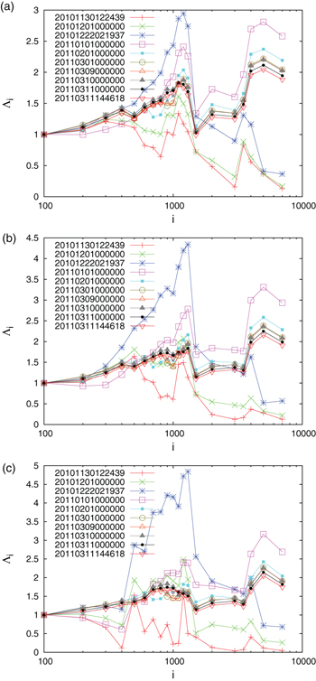
Fig. 2: Plot of  values vs. the scale i (number of events) for all
  EQs in the entire Japanese region
  since 1 September 2010 (a), 1 October 2010 (b), and 1 November 2010 (c). The
  values have been calculated for each scale up to the following ending dates: 30 November 2010 (pluses in red, just before the M7.1 EQ on this date), 1 December 2010 (crosses in green), 22 December 2010 (asterisks in blue, just before the M7.8 EQ that occurred on this date), 1 January 2011 (open squares in magenta), 1 February 2011 (solid squares in cyan), 1 March 2011 (open circles in olive green), 9 March 2011 (open triangles in orange, at 00:00 LT, thus almost 12 hours before the M7.3 EQ occurrence on 9 March 2011), 10 March 2011 (gray filled triangles, at 00:00 LT thus almost 12 hours after the M7.3 EQ occurrence on 9 March 2011), 11 March 2011 (solid circles in black, at 00:00 LT, thus almost 15 hours before the mega-earthquake occurrence) and 11 March (inverted red triangles, almost 10 min before the M9 Tohoku EQ occurrence). The time format in the figure keys is YYYYMMDDhhmmss in Japan Standard Time.
Download figure:
Standard image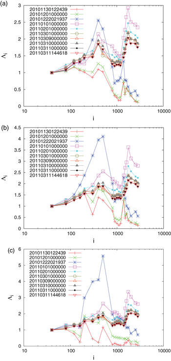
Fig. 3: The same as fig. 2, but here we calculate  values by condidering all
  EQs in the entire Japanese region
  . Only for scales around 800 events or longer the feature described in the text is observed.
Download figure:
Standard imageA close inspection of fig. 2 reveals that for each  events or longer, the
  values after 1 January 2011, which is a date very close to the initiation of the SES activity (thus long-range temporal correlations between EQ magnitudes develop, as mentioned) reach a maximum and afterwards show a systematic decrease until the mainshock occurrence. This behavior persists when starting the computation, either on 1 January 2010 or 1 March 2010, or 1 May 2010, or 1 July 2010, see figs. 1(a) and 3 for
  EQs of ref. [13]. Almost the same behavior is observed in fig. 3 for
  EQs (see also fig. 2(a) of ref. [13]).
The results obtained when considering all  EQs in the entire Japanese region, depend on the date we start. In particular, if the computation starts appreciably earlier in the past, thus fewer events are close to the mainshock occurrence, the aforementioned systematic behavior
  is lost, see fig. 1(b) of ref. [13] for
  when we start the calculation on 1 January 2006. In summary, the results dictate that only when starting the computation close to the impending mainshock, the
  values maximize (cf. such a maximization can be clearly seen in fig. 4 of ref. [13]) upon approaching the date of the SES activity and afterwards start to systematically diminish as we move closer to the mainshock occurrence.
The above behavior of the time evolution of the  values of seismicity in the entire Japanese region, however, is distinctly different from that in the future epicentral area, because
  in the candidate epicentral area exhibits an abrupt increase [13] after the M7.3 EQ occurrence on 9 March 2011 up to the M9 EQ occurrence (cf. more details on this
  increase are given in refs. [13] and [51]), while
  in the entire Japanese region gradually diminishes until the M9 Tohoku EQ occurrence on 11 March 2011. This constitutes the key difference emerged from natural time analysis pointing to the characterization of the M7.3 EQ as a foreshock well in advance and in addition serves for the identification of the occurrence time of the M9 mega-earthquake on 11 March 2011, which is the largest-magnitude event ever recorded in Japan. This is consistent with the fact [20] that the
  values of seismicity after 5 January 2011 in the future epicentral area [35] converged to 0.070 almost a day after the occurrence of the M7.3 EQ, thus revealing again that it was a foreshock.
Conclusion
Upon employing natural time analysis, several EQ precursory phenomena emerge, as described above. These facts obviously invalidate the claim that "earthquakes cannot be predicted", which appeared in the 1990s after the seminal work of Bak et al. on SOC.