


Abstract
We study the motion of a classical particle subject to anisotropic harmonic forces and constrained to move on the  sphere. In the integrable-systems literature this problem is known as the Neumann model. We choose the spring constants in a way that makes the connection with the so-called p = 2 spherical disordered system transparent. We tackle the problem in the N → ∞ limit by introducing a soft version in which the spherical constraint is imposed only on average over initial conditions. We show that the Generalized Gibbs Ensemble, constructed with N conserved charges in involution, captures the long-time averages of all relevant observables of the soft model after sudden changes in the parameters (quenches). We reveal the full dynamic phase diagram with four different phases in which the particles' position and momentum are both extended, only the position quasi-condenses or condenses, and both condense. The scaling properties of the fluctuations allow us to establish in which of these cases the strict and soft spherical constraints are equivalent. We thus confirm the validity of the GGE hypothesis for the Neumann model on a large portion of the dynamic phase diagram.
Export citation and abstract BibTeX RIS
Interest in the long-time dynamics of quantum isolated systems has continuously grown since the celebrated quantum Newton's cradle experiment [1], which proved that a quenched one-dimensional Bose gas does not reach standard thermal equilibrium. Soon after, a Generalized Gibbs Ensemble (GGE) was proposed to describe typical observables in the steady state of systems with an extensive number of conserved quantities, say  with
with  , and N the number of degrees of freedom [2,3]. The pertinence of such density matrix was studied in a myriad of different one-dimensional quantum cases where the necessity to focus on quasi-local observables and constants of motion was stressed [4–7].
Although most studies of quenches of isolated systems have focused on quantum systems, non-ergodic dynamics are not specifically quantum: classical integrable systems [8–10] are not expected to reach equilibrium as dictated by conventional statistical mechanics either. One can then ask whether a GGE description could apply to their long-term evolution as well and, if so, under which conditions. Yuzbashyan argued that the Generalized Microcanonical Ensemble (GME), in which the values of all independent constants of motion are fixed, is exact for classical integrable systems [11]. More explicitly, this means long-time averages of the Newtonian dynamics,  , and statistical averages calculated with the flat GME measure,
  , of typical observables coincide (the sums run over all possible configurations). Here,
  are the values of the constants of motion at the initial time t = 0, and constrain the manifold in phase space in which the dynamics occurs. However, this does not ensure that a canonical GGE, of the form
  , could be derived from such a GME, especially in long-range interacting systems in which the notion of a subsystem is not straightforward and the additivity of the conserved quantities is not justified [12,13]. It is therefore of paramount importance to explicitly construct the GGE of a classical integrable interacting model (beyond the independent harmonic-oscillator case) and put to the test its main statement, that in the stationary limit
1
the long-time average,
, could be derived from such a GME, especially in long-range interacting systems in which the notion of a subsystem is not straightforward and the additivity of the conserved quantities is not justified [12,13]. It is therefore of paramount importance to explicitly construct the GGE of a classical integrable interacting model (beyond the independent harmonic-oscillator case) and put to the test its main statement, that in the stationary limit
1
the long-time average,  , and the phase space average,
  , coincide (for any not explicitly time-dependent and non-pathological observable A). The parameters
  are Lagrange multipliers fixed by requiring that the phase space averages of the N constants of motion,
  , equal their values at the initial conditions,
  . For an early discussion of the GGE for a classical system see [14], and for an approach based on generalized hydrodynamics see [15,16].
Our goal here is to exhibit one such non-trivial classical model, the Neumann Model. We used a mixed analytic-numerical treatment to prove that in the thermodynamic limit, N → ∞, taken before the long-time limit,  , with
  a characteristic time-scale, the model reaches a stationary state which satisfies the extended ergodic hypothesis with a GGE measure in which the
  are integrals of motion in involution (with quartic dependencies on the phase space variables) [17]. In so doing, we elucidated the dynamic phase diagram and we evidenced condensation phenomena and macroscopic fluctuations that should be of importance, as we explain, in quenches of Bose-Einstein condensates.
The Neumann Model (NM) is a non-trivial classical integrable system [18] that describes the motion of a particle on a sphere embedded in an N-dimensional space,  , under fully anisotropic harmonic forces. The Hamiltonian is

with  ,
,  , the coordinates of the position vector,
  the corresponding momentum components, m the mass, and
  the spring constants. The primary and secondary spherical constraints are

The equations of motion, subject to the constraints (2) can be derived with the Poisson-Dirac method and read

The "Lagrange multiplier" z is given by

makes the μ-modes interact, and ensures the validity of C1 and C2. For any initial condition satisfying these constraints, the dynamics conserve them, the quadratic Hamiltonian,  , as well as the N Uhlenbeck integrals of motion in involution [19–22],

The latter verify  , and
, and  , which equals
  thanks to the constraints in eq. (2).
We are interested in developing a statistical description of the NM dynamics. This can make sense only in the limit N → ∞ taken before any long-time limit. In this setting one can expect the fluctuations of z to be suppressed, and

where we made the time dependency of z explicit. The angular brackets represent an average over any distribution of initial conditions satisfying the constraints C1 and C2. The replacement in eq. (6) is a kind of mean-field approximation that softens the strict conditions on C1 and C2 and imposes them on average,  and
and  . In this way, we introduce a variation of the original model that we call the Soft Neumann Model (SNM). With the replacement of the phase space function z by its average, the equations of motion (3) are reduced to those of a system of harmonic oscillators with frequencies

As already said, this model satisfies both constraints only on average over initial conditions. Similarly, it has no strictly conserved quantities but

are also conserved on average. The conditions under which the NM and SNM are equivalent will be analyzed below.
Quadratic potential energies combined with a global spherical constraint as the one in eq. (1) are common in statistical physics. Depending on the choice of the spring constants  one finds, e.g., the celebrated spherical ferromagnet [23,24] or the so-called p = 2 disordered spherical model [25,26]. Problems of particles embedded in large-dimensional spherical spaces and subject to random potentials can also be of this kind. For convenience, and to make a closer connection with the physics of disordered systems, we order the λ's such that
  and in the large N numerical applications we take them to be distributed by a Wigner semi-circle law on the interval
 ![$[-2J,2J]$](https://content.cld.iop.org/journals/0295-5075/132/5/50002/revision2/epl20382ieqn30.gif) . In this way, they can be thought of as the eigenvalues of a two-body interaction matrix with zero-mean Gaussian-distributed entries that couple the coordinates in a different basis (e.g., real spins with a global spherical constraint). The fact that they take values within a real interval with an edge ensures that the total energy is bounded from below. We expect to find similar results for other choices of the distribution of λ's with an edge in the N → ∞ limit.
. In this way, they can be thought of as the eigenvalues of a two-body interaction matrix with zero-mean Gaussian-distributed entries that couple the coordinates in a different basis (e.g., real spins with a global spherical constraint). The fact that they take values within a real interval with an edge ensures that the total energy is bounded from below. We expect to find similar results for other choices of the distribution of λ's with an edge in the N → ∞ limit.
In most studies of quantum quenches, the initial condition is taken to be the ground state of a Hamiltonian which is suddenly modified. However, equilibrium finite-temperature initial states [27–30] are more relevant to describe, for instance, experiments in ultracold Bose gases [31]. Along these lines, we draw the initial conditions from a proper Gibbs-Boltzmann equilibrium measure

where  is the equilibrium value of the Lagrange multiplier enforcing the spherical constraint (also on average) at inverse temperature
  with
with  .
.  is the canonical partition function, and
  is given in eq. (1) with spring constants
  in the interval
 ![$[-2J_0, 2J_0]$](https://content.cld.iop.org/journals/0295-5075/132/5/50002/revision2/epl20382ieqn37.gif) . The equilibrium
. The equilibrium  takes the values

Depending on  being larger or smaller than one, the initial conditions belong to an extended phase in which the variances of all modes are
  , or to a condensed phase in which the averaged squared N-th mode,
  , scales as
  [25]. Two scenarii for the condensation phenomenon are possible: a mixed two-pure-state measure with the possibility of symmetry breaking induced by a vanishing pinning field, or a Gaussian measure centered at zero with diverging dispersion [24,32,33]. In the magnetic interpretation,
  is a critical point between a disordered and a magnetically ordered phase. The analogy with Bose-Einstein Condensation (BEC) was already reckoned in [25] with
  playing the role of the ground state density. The transition, in this case, is towards the condensed phase.
We drive the system out of equilibrium by performing a sudden interaction quench in which we rescale all spring constants,  , with the same factor
  that controls the amount of energy injected (
 ) or extracted (
 ). This procedure mimics the quenches performed in isolated quantum systems [4–6]. Right after the instantaneous quench, the initial kinetic energy of all modes is
  and the averaged Uhlenbeck constants are
  for
for  while
while  for
for  . Each
  is a function of
  and the adimensional parameters
  and
and  that can be easily calculated:

for  or
or  and
and  , and
, and

for  .
.
Insight into the long-time dynamics of the SNM was gained in [14,34]. In these papers we studied the Schwinger-Dyson equations that couple the global two-time correlation, C, and linear response, R, averaged over the initial measure  and, also, the harmonic spring constants (quenched randomness), in the strict N → ∞ limit. This approach bears resemblance with dynamic mean theory [35]. The (replica) method used to impose the thermal initial conditions ensures symmetry breaking for
  . Four phases were identified in the
  phase diagram (energy injection/initial condition characteristics) as deduced from
  , which equals
  for
for  (II, III) and
  for
for  (I, IV), and
  , which takes a non-zero value for
  and
and  (III), see fig. 1. The asymptotic value of the Lagrange multiplier is strictly larger than
  for
for  , whereas it locks to
  for
for  implying that the potential on the N-th mode flattens and the gap of the effective Hamiltonian closes for t → ∞ after N → ∞. Noteworthy, all these observables approach constant limits algebraically with superimposed oscillations [34].
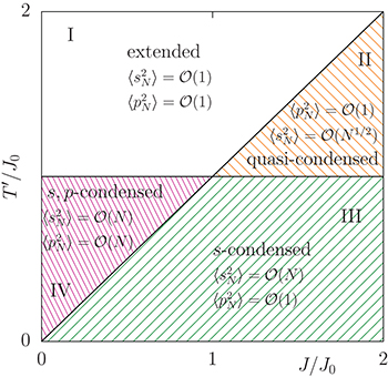
Fig. 1: The dynamic phase diagram.  and
and  to the left of the diagonal (I, IV), and
  and
and  to the right of it (II, III).
  in III and vanishes elsewhere. The names of the phases refer to the condensation phenomenon arising in III and IV, see the explanation in the text. The averages
  represent either GGE or dynamic ones, since they coincide in the asymptotic limit taken after the large N limit. All transition lines are continuous.
Download figure:
Standard imageIn this letter we work with a fixed (and typical) realization of the  . On the one hand, we solve the coordinate dynamics for finite but large N and, ideally, long times with a modification of the semi-analytic phase-Ansatz method used in [36] to study the O(N) field theory, and adapted in [14] to the present case. With this method we compute the time averages
  and
and  (controlling the deviations from the ideal limit t → ∞ after N → ∞). The particle's behaviour in each Sector of the phase diagram of fig. 1 is sketched in fig. 3. In Sector I the particle is delocalised on the full sphere initially and it remains like this subsequently. In Sector II, the initial extended state with negligible projection on the N-th mode develops into configurations with a sub-extensive projection on this particular direction. In Sector III, the motion remains condensed, similarly to how it was initially. Finally, in Sector IV the N-th mode acquires extensive kinetic energy. More quantitative details are given later, when we compare dynamic and GGE averages.
On the other hand, we calculate the GGE partition sum

with  ,
,  and
and  the Lagrange multiplier that imposes the spherical constraint (which in this formulation could be reabsorbed in the definition of
  thanks to
  ). The standard Gibbs-Boltzmann equilibrium partition sum (relevant to describe the case
  and any
  ) is recovered by setting
  and
and  . We evaluate the averages
  and
and  that we compare to the dynamic ones
  and
and  . We analyze the fluctuations of the constraints C1, 2 (dynamically and with the GGE) and from their scaling we determine in which cases the SNM is equivalent to the proper NM.
The partition sum  is a non-trivial object since the
  are quartic functions of the phase space variables, see eq. (5). Still, we managed to calculate it by adapting methods that are common in the treatment of disordered systems and random matrices [17]. Firstly, we used auxiliary variables to decouple the quartic terms. Secondly, for N → ∞, we transformed
  into a continuous variable λ, all
  into
into  for any
  , and
, and  with
with  the Cauchy principal value. In both integrals
  is the density of spring constants taken to be of Wigner form. In some cases we separated the contribution of the N-th mode which may be macroscopic and scale differently from the ones in the bulk. Thirdly, we evaluated
  by saddle-point. Then, we showed that the harmonic Ansatz

solves the saddle-point equations. Finally, we exploit the conditions  , with
  evaluated at the saddle point to close the system of equations. In the absence of initial condition condensation,
  , all Uhlenbeck constants are
  and their GGE averages should equal the ones over initial conditions given in eq. (11)

When the initial state is condensed,  , eq. (15) applies to all λ with the exception of
  , for which

plus o(1) corrections, and  given in eq. (12). Together with the constraint
  , these are the central equations that allow us to solve the problem. Their numerical solution yields the spectrum of mode temperatures,
  ,
,  and
and  , and with them we deduce the expectation value of any observable. A selected number of results are shown in fig. 2 where we compare the GGE averages to the dynamic ones for parameters in Sectors I and IV of the phase diagram displayed in fig. 1. We collect dynamic data for N = 100, 1024 and GGE data for N = 100 (with a more naive saddle point evaluation) and N → ∞. The agreement is very good. The rather small extent of finite size effects in the bulk can also be appreciated in the figure (the double logarithmic scale enhances the appearance of the deviations, which are actually restricted to the neighborhood of the edge in (c) and (d)). In the insets in (a) and (c) the spectra of the Lagrange multipliers
  for finite N are shown, which can be compared to the one of
  . Results of similar quality are obtained in Sectors II and III (not shown).
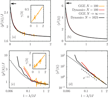
Fig. 2: The dynamic and GGE averages of  and
and  against
  in Sectors I
  (a) and (b), and IV
  (c) and (d), of the phase diagram. In the insets the parameters
  . The arrows in (a) and (b) indicate the finite values of
  and
and  at the edge of the spectrum, contrary to their divergence in (c) and (d) (note the double logarithmic scale). In (d) the dotted line is a guide to the eye to an approximate algebraic behavior in the bulk. The N → ∞ GGE averages were computed as explained in the text while the finite N ones were derived using a naive saddle-point evaluation of
  .
.
Download figure:
Standard imageThe dynamics in each Sector and the equivalence between the NM and the SNM can be rationalized according to the scaling properties of the last mode and the fluctuations of the constraints

which can be studied both dynamically and with the GGE. When the scaling of these fluctuations is  the SNM is not equivalent to the NM.
In Sector I,  and
and  are
are  for all μ, including
  . In a sense, this is the simplest possible generalization of the Boltzmann equilibrium extended phase. In Sector II, we have numerical evidence for
  scaling as
  , while
  and
and  should be
  . This is a quasi-condensed phase in which the weight of the last mode is large but not extensive. Since there is no condensation, the energy conserving dynamics in the extended and quasi-condensed phases explore the full sphere in the course of time as sketched in figs. 3(a), (b) with a red dot and the red sphere, respectively. Moreover,
  and the NM and SNM models are equivalent in Sectors I and II.
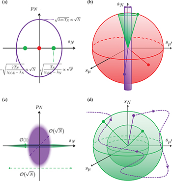
Fig. 3: Sketches of particle trajectories in the extended (I) and quasi-condensed (II) phases in red, s-condensed (III) in green and s, p-condensed (IV) in violet. In (a) and (c) we show the averaged and fluctuating N-th mode plane, respectively, and in (b) and (d) the motion in the N-dimensional coordinate space. The dynamics in (a) and (b) use extended ( , I-II) and symmetry broken (
 , III-IV) initial conditions. Panels (c) and (d) illustrate the violations of the constraints Ci
due to the condensation of fluctuations for initial conditions with macroscopic fluctuations of sN
(III-IV).
, III-IV) initial conditions. Panels (c) and (d) illustrate the violations of the constraints Ci
due to the condensation of fluctuations for initial conditions with macroscopic fluctuations of sN
(III-IV).
Download figure:
Standard imageIn Sectors III and IV, where the initial conditions are drawn from the Boltzmann measure of the SNM at  . As explained above, they can be of two kinds: i)
  with negligible fluctuations, or ii)
  Gaussian distributed, centered at zero with
  fluctuations [24,32]. In both cases
  , but the dynamics are different and have to be discussed separately.
In case i), Sector III is a properly s-condensed phase with  scaling as N, while
  and
and  . The system precesses around one of the two states with
  , the one selected by the symmetry-broken initial conditions, and comparably negligible projection on all other directions, see the symmetrically placed green dots and green trajectory in figs. 3(a), (b), respectively. The constraints C1 and C2 are strictly satisfied up to sub-extensive corrections and the NM and SNM are equivalent. Remarkably, in Sector IV both
  and
and  scale as N, and the N-th mode captures
  kinetic energy. We call this Sector an s, p-condensed phase. The last mode is in a superposition of states associated to each initial condition. At any instant t, the configurations are distributed on an ellipse in the plane (sN
, pN
) with axes
kinetic energy. We call this Sector an s, p-condensed phase. The last mode is in a superposition of states associated to each initial condition. At any instant t, the configurations are distributed on an ellipse in the plane (sN
, pN
) with axes  , as in the closed motion of a harmonic oscillator, see the violet ellipse and cylinder in figs. 3(a), (b), respectively. The average over trajectories implies, in particular, that the limit correlation q0 vanishes. The constraints C1, 2 are only verified on average over the initial conditions and the SNM and NM are not equivalent. We note that
  are averages of a quartic functions of the phase variables; had we evaluated only quadratic functions of sN
we would have not noticed the inequivalence between the two models. Quite surprisingly, the averaged dynamics cannot be boiled down to the ones of a typical trajectory with its own z(t).
are averages of a quartic functions of the phase variables; had we evaluated only quadratic functions of sN
we would have not noticed the inequivalence between the two models. Quite surprisingly, the averaged dynamics cannot be boiled down to the ones of a typical trajectory with its own z(t).
In case ii), the initial conditions imply  at all times due to the large fluctuations of the last mode. One can show that, in Sector III,
  at all times. In this situation, due to the large fluctuations in C1, zero-mean initial conditions are appropriate for the soft model but not for the strictly spherical one. In practice, in the SNM we average over spherical trajectories with different radius determined by the initial condition. In Sector IV, due to the condensation of pN
, the dynamics do not preserve the scaling properties of C2 either. In other words, the fluctuations of the secondary constraint, which vanish in the initial condition, get macroscopically amplified by the dynamics. In conclusion, we average over trajectories that no longer move on the sphere. In this Sector, the fluctuations of all the quantities that are conserved on average,
at all times. In this situation, due to the large fluctuations in C1, zero-mean initial conditions are appropriate for the soft model but not for the strictly spherical one. In practice, in the SNM we average over spherical trajectories with different radius determined by the initial condition. In Sector IV, due to the condensation of pN
, the dynamics do not preserve the scaling properties of C2 either. In other words, the fluctuations of the secondary constraint, which vanish in the initial condition, get macroscopically amplified by the dynamics. In conclusion, we average over trajectories that no longer move on the sphere. In this Sector, the fluctuations of all the quantities that are conserved on average,  , C1, 2 and IN
, condense, which implies that the dynamics do not conserve the quadratic energy, are not restricted to a sphere and are not strictly integrable. The behaviours in Sectors III and IV are represented in figs. 3(c), (d), with the same colour code as the one we used before.
, C1, 2 and IN
, condense, which implies that the dynamics do not conserve the quadratic energy, are not restricted to a sphere and are not strictly integrable. The behaviours in Sectors III and IV are represented in figs. 3(c), (d), with the same colour code as the one we used before.
Contrary to the quantum mechanical subtleties [37,38], the notion of classical integrability is clear [8–10]. The dynamics should be ergodic on the portion of phase space compatible with the constants of motion [11]. Still, the fact that a canonical GGE could describe the time-averages of generic observables in a classical interacting integrable system is not obvious. We modified the celebrated Neumann model by imposing the spherical constraint on average over the initial conditions and we were then able to solve it in the thermodynamic limit. We thus provided an explicit example in which identities between temporal and statistical averages, for all kinds of thermal initial conditions (on average) and observables not correlated with the constants of motion and post-quench parameters, can be demonstrated.
Importantly enough, for condensed initial states,  and
and  are macroscopic and stay so after the quench. In these cases, we distinguished symmetry-broken initial conditions and symmetric ones with zero mean and condensed fluctuations. Quadratic observables are insensitive to the changes that the latter induce but quartic ones are not. For symmetry-broken initial conditions, the SNM behaves just as the NM in the phase in which only the coordinate is condensed but it loses its equivalence with the NM in the phase in which not only the coordinate but also the momentum condenses. For initial states with macroscopic fluctuations, although the dynamics conserve on average an extensive number of phase space functions, the individual trajectories do not. Energy conservation is violated in the condensed Sectors of the phase diagram and the SNM and NM are not equivalent. Interestingly enough, given the similarity between the phase transitions and condensation in this model and in BEC [25,33] we may expect similar phenomena in quenches of thermal initial states of the latter.
In conclusion, we provided a new class of classical integrable systems in which the stationary dynamics is captured by the GGE measure. Notice that the integrals of motion in the NM and SNM are non-local, in the sense that the  are given by sums involving all coordinates and associated momenta. These models are, therefore, different from the one-dimensional cases, with (quasi)-local constants of motion, that are usually dealt with in equilibration studies of integrable systems.
Acknowledgments
We thank J.-B. Zuber for very helpful discussions.
Footnotes
- 1
The time
 is the time-scale needed to reach stationarity and it will typically be much longer than a microscopic time-scale t0.
