

Abstract
We present a numerical study of horizontal convection using both step and linear forcing profiles as the imposed surface thermal driving, the former of which is commonly used in many studies but the latter is closer to the real ocean. Our investigation focuses on how forcing profiles can affect the theoretical and experimental results previously obtained based on the step forcing profile. We show that both types of forcing profiles exhibit similar behaviors in terms of global heat transfer (Nu), mean flow strength (Re), and boundary layer thickness. However, these two forcing profiles show significant differences for some other physical quantities, such as the generation rate of available potential energy GAPE and global thermal dissipation rate, for which exact relationships with Nu can be derived for the step forcing profile but not for linear forcing. We show that a relationship between Nu and GAPE can be developed for linear forcing by defining an effective forcing area, and such area is found to be approximately constant. We further derive an approximate relationship between Nu and the global thermal dissipation rate for linear forcing by assuming that the boundary heat flux is proportional to the local temperature deviation from the mean, which works best under the condition of moderate plume emissions. Differences are also found for the viscous dissipation rate; however, these differences diminish for sufficiently high Ra. Though step forcing is obviously less appropriate for modeling ocean circulations, we show that most differences arising from the forcing profile difference can be reconciled. Considering its convenience in experiment control and theoretical analysis, step forcing is a good configuration for most problems, but one should also be aware of the differences between step and other forcing types in quantities like the global thermal dissipation rate when extrapolating the results to more general situations.
Export citation and abstract BibTeX RIS
Introduction
The meridional overturning circulation (MOC) plays a crucial role in the Earth's climate and energy system [1–4]. Potential candidates for the MOC energy sources include wind and tide [5], geothermal heating [6], and surface thermal forcing. An important conceptual model in the study of the effect of surface thermal forcing is horizontal convection (HC), in which the flow is driven by the surface temperature difference applied horizontally on a fluid layer [6–12]. There are two dimensionless control parameters in this system:  is the Rayleigh number representing the strength of thermal driving, and
  is the ratio between momentum and thermal diffusivity of the working fluid. Here α is the thermal expansion coefficient, g the gravitational acceleration,
  the temperature difference between hot and cold plates, L the length of the convective cell, ν refers to the kinetic viscosity, and κ the thermal diffusivity. Nusselt number Nu and Reynolds number Re are two of the main responding parameters of this system. The Nusselt number is defined as
  , where
  represents the averaging over time and the surface with non-zero heat flux. The Reynolds number is defined by
  , where U is the characteristic velocity of the system. A recent study [11,13] extended the Grossmann and Lohse (GL) theory for the Rayleigh-Bénard convection [14–17] to HC and revealed various scaling laws of Nu and Re with Ra based on the step forcing profile, in which the hot and cold plates take up a fraction of the top (or bottom) surface and each with uniform temperature are located at the two ends of the cell. For
  , a scaling relationship
  is predicted when Ra is low (denoted by the I*
lregime). In this regime, the boundary layer dominates the global heat transport and the viscous boundary layer thickness is a constant of the order of the cell height [11,15]. As Ra increases, the Rossby scaling [7] can be obtained (also denoted by Ilin refs. [11,13]), in which the heat transport is dominated by the boundary layer. For sufficiently high Ra such that the heat transport is controlled by the bulk flow, a scaling relationship
is predicted when Ra is low (denoted by the I*
lregime). In this regime, the boundary layer dominates the global heat transport and the viscous boundary layer thickness is a constant of the order of the cell height [11,15]. As Ra increases, the Rossby scaling [7] can be obtained (also denoted by Ilin refs. [11,13]), in which the heat transport is dominated by the boundary layer. For sufficiently high Ra such that the heat transport is controlled by the bulk flow, a scaling relationship  was predicted (corresponding to the IVuregime in ref. [11]). In ref. [18], the authors proposed a similar 1/4-scaling when the bulk flow is significantly turbulent. In that study, a HC system with spatially periodic thermally forcing was used. The transition to
  was observed when the scales of turbulent motion exceed the forcing scale and become comparable to the width of the box.
There is no standard choice for the type of forcing profile for horizontal convection, per se. Thus, various forcing profiles have been used in studies of HC, which include step, linear [19], sinusoidal [18,20–22], and mixed profile of fixed heat flux and fixed temperature [9]. Because of experimental and theoretical convenience, the step forcing profile has become the most frequently used in the studies of the HC system [6,11–13,23–27].
However, step forcing is obviously less relevant to the real ocean when compared with other types of forcing profiles with continuously varying temperature along the surface. To apply the results obtained based on step forcing profiles to the other types, it is important to know how the key quantities of the flow will be affected. Tsai et al. [28] compared the influence that different forcing profiles have on the global heat transfer and on the transitional behaviour of the system to the turbulent state. They proposed that the linear forcing profile gives a power law scaling closer to  than that given by step forcing, and forcing profiles can induce different transitional behaviour from laminar to turbulent flow. However, how some of the important quantities, such as the Reynolds number, the boundary layer thickness, and the generation rate of available potential energy, behave under the different profiles remains to be explored. To find out such differences, we have conducted a comparative study of the step and continuous forcing profiles. Among different continuous forcing profiles, we use linear forcing in this study, which can already illustrate the main differences with the step forcing.
Numerical setup
In this study a series of three-dimensional direct numerical simulations (DNS) are conducted. We consider a body of fluid (water in the present case) with non-slip boundary conditions at all boundaries. All lateral and bottom boundaries are adiabatic. As illustrated in fig. 1, the temperature difference driving the system is applied on the top surface. We use two kinds of thermal forcing profiles: a) Step forcing profile. In this configuration, the top surface is divided into three regions, a hot plate at one end and a cold plate at the other end. Each plate takes up 1/10 of the length of the top surface, with the remaining part of the surface being adiabatic. The hot and cold plates have uniform temperature Thot
and Tcold
, respectively. b) Linear forcing profile, in which the temperature is linearly distributed over the length of the entire top surface, i.e.,  . The geometrical properties of the convective cell is characterized by the aspect ratio
  , where H is the height of the convection cell. The system is governed by Navier-Stokes equations in the Oberbeck-Boussinesq approximation

where  , u, p and
 ![$\theta=[T-(T_{hot}+T_{cold})/2]$](https://content.cld.iop.org/journals/0295-5075/135/2/24006/revision2/epl21100319ieqn15.gif) are the mean density, velocity, pressure and reduced temperature, respectively. The governing equations (1) are solved in a dimensionless form. We non-dimensionalized the equations using
are the mean density, velocity, pressure and reduced temperature, respectively. The governing equations (1) are solved in a dimensionless form. We non-dimensionalized the equations using  ,
,  ,
,  and
and  .
.

Fig. 1: Illustrations of the numerical setup. (a) Step forcing profile, and (b) linear forcing.
Download figure:
Standard imageWe conduct the simulations using a DNS code called CUPS [29–31], which is based on the finite-volume method and achieves 4th-order spatial precision. Temperature and velocity fields are discreted in staggered grids. The characteristic lengths of temperature and velocity are the Batchelor and the Kolmogorov length scale, respectively. For Pr > 1, the Batchelor length scale is smaller than the Kolmogorov length scale. In the traditional single resolution scheme, only one set of meshes is used. To ensure that both momentum and temperature fields are resolved, the meshes to be used are required to resolve the smallest length scale in the system, i.e., the Batchelor length scale. This scheme will inevitably bring some unnecessary computational costs in the momemtum solver. In the multiple resolution scheme, the momemtum and temperature fields are solved in their respective set of meshes, so that only the meshes for the temperature field needs to resolve the Batchelor length scale and the momentum field can be solved in coarser meshes. Thus, computational costs can be efficiently saved without any sacrifices in precision [31]. For simulations with  , the multiple resolution scheme is used; while for
  we use the single resolution method. Lists of the meshes used in our simulations and other statistical quantities are provided in the Supplementary Material Supplementarymaterial.pdf . Tests have been done comparing global quantities of the system, e.g., Nu, and we find that the differences between two numerical methods are within 1%. To ensure that small local length scales are resolved, grids are refined near boundaries. For the step forcing profile, the normalized total area of hot and cold plates, denoted as
  , is fixed to be 0.1. We fixed
  and
and  in this study, and varied Ra from
  to
to  .
.
Results
We first discuss and compare our results of Nu with other studies. In fig. 2(a), we present Nu compensated by Ra0.23, which is the scaling relationship we observed for both forcing profiles after plume emissions occur. This scaling relationship agrees with the results for high Pr observed in refs. [13,23,24]. For comparison, we also plot the results from refs. [23,24], which use step forcing and the same configuration and geometry as ours. Here we only use those with Pr = 10 from their results, which is the closest Pr to ours. The results of both step and linear forcing in ref. [28] for  ,
,  and
and  are also plotted in fig. 2(a). As shown in fig. 2(a), our results for the step forcing profile agree well with those of refs. [23,24]. Comparing our results with those of ref. [28], we find that for
  both data sets yield similar scaling behavior for both step and linear forcing. However, there exist significant differences in the magnitudes of Nu for linear forcing and scaling relationships at
  for both forcing types. Such differences may be attributed to the different Γ used in the two studies.
For linear forcing, heat transfer is less efficient in the middle part than in the two ends, since the temperature contrast between the the top plate and the bulk flow is small in the middle. When evaluating Nu, the whole top plate is taken into account for linear forcing, which makes the magnitudes for linear forcing overall smaller than the step forcing, as shown in fig. 2(a). For  a steep scaling is observed. As Ra increases, we observe the Rossby scaling
  [7,11] for about a decade
  for both forcing profiles. For
  , plume emissions occur and a scaling relationship
  is observed. However, the transitional behaviour between linear and step forcing appears to be different, i.e., for step forcing the system directly changes from the Rossby scaling
  to
to  at
at  , but for linear forcing a gradual transition is observed. Nevertheless, for both profiles the system shows a clear
  scaling relationship when Ra reaches
  . Moreover, though Tsai et al. [28] argued that the linear forcing profile gives a power law scaling relationship closer to
  than the step one, we find that the difference in scaling between step and linear forcings is actually insignificant for their results with both being close to
  for high Ra.
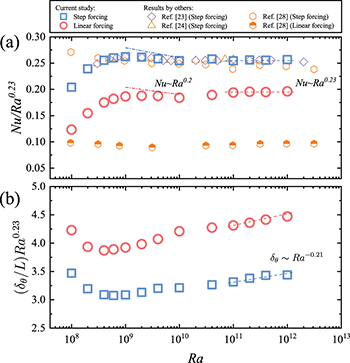
Fig. 2: (a) Nu compensated by Ra0.23, and (b) thermal boundary layer thickness  normalized by
  for two types of forcing profiles.
Download figure:
Standard imageThe thermal boundary layer thickness  has a deep connection with Nu. The relationship between Nu and
  can be written as

where Tbulk
is the bulk temperature. For Rayleigh-Bénard convection (RBC), since  , the thermal boundary layer thickness is usually given by
  . This approximation has also been applied to the HC system [11–13]. To examine this approximation, we measure the thermal boundary layer thickness
  for both forcing profiles. The thermal boundary layer thickness is first measured locally using the slope method [32] and then averaged over
  for both forcing profiles. The results of
  compensated by
  are shown in fig. 2(b). One can observe that for
  ,
,  follows a less steep scaling relationship than
  (we observe
  ), suggesting that
  does not follow the assumption
  . In the HC system, plume emissions occur only in the vicinity of the cold plate and the cold downwelling flow is dominant. For this reason, Tbulk
is closer to Tcold
than Thot
. As Ra increases, the cold plumes emit more frequently, which further decreases Tbulk
. Thus, the prefactor
. In the HC system, plume emissions occur only in the vicinity of the cold plate and the cold downwelling flow is dominant. For this reason, Tbulk
is closer to Tcold
than Thot
. As Ra increases, the cold plumes emit more frequently, which further decreases Tbulk
. Thus, the prefactor  in (2) increases as Ra increases, which makes the Ra dependence of
  being less steep than
  . Nevertheless, as Ra further increases and the bulk temperature becomes sufficiently close to the cold plate, the dependence of the bulk temperature on Ra becomes much weaker than in low Ra, and it would then be valid to assume
  .
.
We next discuss the results of the Reynolds number for the two forcing profiles. Two kinds of characteristic velocities Umax
and Uke
are used to evaluate Re. Umax
is obtained by taking the average value of the local maximum ux
over the region ![$x/L\in[0.2,0.8]$](https://content.cld.iop.org/journals/0295-5075/135/2/24006/revision2/epl21100319ieqn64.gif) . Figure 3(b) shows examples of the ux
profiles at three representative positions. We use Umax
here because it may be used to characterize the velocity of the thermocline in the context of oceanic circulations [33]. We remark here that from fig. 3(b) it is clear that the convective flow is mostly confined to the upper half of the convection layer, i.e., the circulation is shallow. This is consistent with a previous experimental observation that convective flows in HC do not penetrate deep into the convection cell [27]. Uke
is defined according to the mean kinetic energy of the system
. Figure 3(b) shows examples of the ux
profiles at three representative positions. We use Umax
here because it may be used to characterize the velocity of the thermocline in the context of oceanic circulations [33]. We remark here that from fig. 3(b) it is clear that the convective flow is mostly confined to the upper half of the convection layer, i.e., the circulation is shallow. This is consistent with a previous experimental observation that convective flows in HC do not penetrate deep into the convection cell [27]. Uke
is defined according to the mean kinetic energy of the system  . Corresponding to these two velocities, two Reynolds numbers can be defined:
  represents the flow stength of the thermocline, and
  indicates the mean flow strength of the system. We present the obtained Reke
and Remax
in fig. 3(a). The results for Reke
for Pr = 10 in ref. [23] are also shown in fig. 3(a) for comparison, which show good agreement with the present ones. Multiple transitions can be seen for both Reke
and Remax
. These transitions are consistent with those in Nu –Ra shown in fig. 2(a). For
indicates the mean flow strength of the system. We present the obtained Reke
and Remax
in fig. 3(a). The results for Reke
for Pr = 10 in ref. [23] are also shown in fig. 3(a) for comparison, which show good agreement with the present ones. Multiple transitions can be seen for both Reke
and Remax
. These transitions are consistent with those in Nu –Ra shown in fig. 2(a). For  , one can observe very similar behaviour in both Remax
and Reke
for the two forcing profiles. After a steep scaling corresponding to the
, one can observe very similar behaviour in both Remax
and Reke
for the two forcing profiles. After a steep scaling corresponding to the  regime in refs. [11,13] for small Ra, a scaling relationship
  can be observed for both Remax
and Reke
when Ra increases. This scaling relationship agrees with the predictions in ref. [9] and the Il
(boundary layer dominating) regime in refs. [11,13]. When Ra further increases, the transition in the Re –Ra scaling can be observed for both Reynolds numbers. In this regime, Reke
and Remax
give different scaling exponents. For the former, we observe a scaling relation close to
can be observed for both Remax
and Reke
when Ra increases. This scaling relationship agrees with the predictions in ref. [9] and the Il
(boundary layer dominating) regime in refs. [11,13]. When Ra further increases, the transition in the Re –Ra scaling can be observed for both Reynolds numbers. In this regime, Reke
and Remax
give different scaling exponents. For the former, we observe a scaling relation close to  , which agrees with ref. [23]. As for the latter, the scaling exponent is approximately 0.44. This exponent is larger than any previous predictions [9,11], suggesting that one may have underestimated the velocity of the thermocline when applying the current theories in HC to the oceanic problems. The difference in the scaling relationship between Remax
and Reke
also suggests the high degree of inhomogeneity in this system. Moreover, the linear forcing produces larger magnitude for both Remax
and Reke
than step forcing, although the difference for Reke
is significantly smaller than that for Remax
. These results also suggest that the type of forcing profiles has stronger influence on the thermocline than it has on the bulk flow.
, which agrees with ref. [23]. As for the latter, the scaling exponent is approximately 0.44. This exponent is larger than any previous predictions [9,11], suggesting that one may have underestimated the velocity of the thermocline when applying the current theories in HC to the oceanic problems. The difference in the scaling relationship between Remax
and Reke
also suggests the high degree of inhomogeneity in this system. Moreover, the linear forcing produces larger magnitude for both Remax
and Reke
than step forcing, although the difference for Reke
is significantly smaller than that for Remax
. These results also suggest that the type of forcing profiles has stronger influence on the thermocline than it has on the bulk flow.
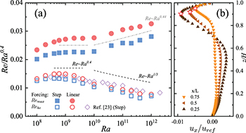
Fig. 3: (a) Re compensated by Ra0.4 for two forcing profiles, and (b) vertical profiles of ux
at  for
for  with step forcing. Stars in (b) represent the ux
with maximum absolute value.
with step forcing. Stars in (b) represent the ux
with maximum absolute value.
Download figure:
Standard imageFrom the above discussions on Nu and Re, one sees that the influence of the forcing profile is mainly on the magnitudes of these quantities. The scaling relations in Nu and Re observed in step forcing profiles are similar to those of linear forcing. In the rest of this paper, we focus on the differences in other quantities for these two forcing profiles.
The available potential energy (APE) is the portion of potential energy that can be converted into kinetic energy [34,35]. The generation rate of APE can be expressed as [34]

where  is the reference position for the state of minimum potential energy of the corresponding fluid parcel. For the step forcing profile,
  equals H at the hot plate and 0 at the cold plate, while for the rest of the cell surface
  . Thus, from (3) we can derive an exact relationship between GAPE
and Nu [12]:
. Thus, from (3) we can derive an exact relationship between GAPE
and Nu [12]:

This exact relation provides a direct connection between heat transfer efficiency and the generation rate of APE. However, for the linear forcing profile,  at the whole top surface, and the local
  depends on the bulk temperature distribution. Thus, one cannot derive an exact relationship between Nu and GAPE
. Since
depends on the bulk temperature distribution. Thus, one cannot derive an exact relationship between Nu and GAPE
. Since  for large Ra, which is the same for both types of forcing profiles, one can find that
  according to (4). To examine the relationship between Nu and GAPE
, we evaluate GAPE
using (3) and show the normalized results in fig. 4. Interestingly, we find that the GAPE
shown in fig. 4 behaves similarly as the compensated Nu plotted in fig. 2(a), although in fig. 4 the normalized GAPE
for linear forcing is larger than that of step forcing. This result suggests that for the linear forcing profile there could exist a relationship that is formally the same as (4). To check this statement, we first define an effective forcing area ratio
according to (4). To examine the relationship between Nu and GAPE
, we evaluate GAPE
using (3) and show the normalized results in fig. 4. Interestingly, we find that the GAPE
shown in fig. 4 behaves similarly as the compensated Nu plotted in fig. 2(a), although in fig. 4 the normalized GAPE
for linear forcing is larger than that of step forcing. This result suggests that for the linear forcing profile there could exist a relationship that is formally the same as (4). To check this statement, we first define an effective forcing area ratio  for linear forcing profile according to

The results of  for linear forcing are shown in the inset of fig. 4, and one finds
  approximately equal to a constant 0.38. With the effective forcing area ratio
  determined, we can estimate GAPE
with Nu according to (5). More importantly, this result suggests a general connection between heat transfer and the generation rate of APE. This connection does not rely on a specific forcing profile. It would be interesting to examine whether
determined, we can estimate GAPE
with Nu according to (5). More importantly, this result suggests a general connection between heat transfer and the generation rate of APE. This connection does not rely on a specific forcing profile. It would be interesting to examine whether  is still a constant for other forcing profiles.

Fig. 4: Normalized GAPE
for two forcing profiles. The inset shows  for the linear forcing profile. The red dashed line represents 0.38.
Download figure:
Standard imageIn the HC system, the rate of change in potential energy  and kinetic energy
  are given, respectively, by [34,35]


Here  is the conversion rate from Ep
to Ek
,
is the conversion rate from Ep
to Ek
,  is the rate of production of Ep
, and
is the rate of production of Ep
, and  is the global viscous dissipation, where
  . Taking the temporal averaging of (6) and (7), one can obtain

The non-dimensionalized visous dissipation (8) is found to be constant for the step forcing profile [13]. In fig. 5(a) we show the normalized dissipation rate for the two types of forcing profiles. It is seen that the normalized viscous dissipation for step forcing is approximately a constant  in our study, which is close to the value of 2 observed in ref. [13]. For the linear forcing, it is clear that the normalized viscous dissipation rate increases with increasing Ra. This result can be understood as follows. From (8) one sees that the normalized viscous dissipation is directly related to the normalized temperature difference between the top and the bottom. For linear forcing, the mean top temperature
  is always zero. On the other hand, the bottom is cooled by the downwelling plumes detached from the cold plate, which becomes colder as Ra increases. Thus, the bottom temperature
  decreases and
  increases as Ra increases for the linear forcing profile, as shown in fig. 5(a). However, since
  , one expects that for sufficiently high Ra,
  approaches to its upper limit 0.5 and becomes insensitive to the change of Ra. In such limiting case, the normalized viscous dissipation will be approximately a constant
  . In the present study,
  is observed for the highest Ra.
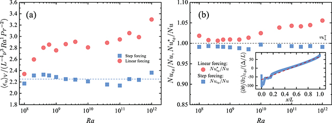
Fig. 5: (a) Normalized viscous dissipation as a function of Ra. The blue dashed line represents a constant 2.25. (b)  for step forcing profile and
  for linear forcing. The inset is the longitudinal distribution of the normalized heat flux on the top surface for linear forcing profile with
  . The red dashed line represents
  .
.
Download figure:
Standard imageBeside the global viscous dissipation, the dissipation rate of temperature variance also shows significant difference for the step and linear forcing profiles. The dissipation rate of temperature variance is given by  . Multiplying (1c) by θ and integrating in time and volume gives

For the step forcing profile, the regions with non-zero  have constant temperature θ, so (9) leads to an exact relation between
  and the mean surface heat flux Nu:

Thus, one can define a Nusselt number using the mean dissipation rate of thermal variance:

As for linear forcing (or other continuous forcings), the coupling between θ and  forbids an exact relation between Nu and
  . To solve this problem, the key is to decouple θ and
  . We assume that the local heat flux is positively correlated to the forcing temperature. For simplicity, we further assume that such correlation is linear, i.e.,
  . Thus, the surface heat flux can be expressed as

By substituting (12) into (9), one obtains the following relation for the linear forcing profile:

From (13) we can find an approximate expression for Nu

The results of  for the linear forcing profile are shown in fig. 5(b). For comparison and verification of our simulations, we also plot
  for step forcing. One sees that for
  agrees well with Nu, suggesting that the linear approximation can properly describe the relationship between θ and
  . As for
  ,
,  increases as Ra increases. To explain this deviation, we first examine the linear approximation (12). We show the longitudinal distribution of the normalized heat flux on the top surface for the linear forcing profile with
  in the inset of fig. 5(b). For the hotter half
  , one can find that the linear approximation (red dashed line) agrees with the actual surface heat flux. However, clear disagreement is seen at the cold end, where the linear approximation significantly underestimates the local heat flux. This is because abounded plumes are emitted at the cold end and enhance the local heat flux there. Since the cold end contributes a large fraction of the global heat transfer, the linear approximation in the model leads to an underestimation in (13). In other words, when plume emissions occur, (13) becomes

Therefore,  , which is proportional to
  according to its definition (14), should be larger than Nu. Since plume emissions become more frequent as Ra increases, the underestimation of local heat flux in the linear approximation of (12) becomes more significant. Thus,
  increases with Ra for
  , as observed in fig. 5(b). This result also implies that for the linear forcing profile the dissipation rate of temperature variance
  should have a stronger Ra dependence than Nu.
Conclusion
In this study we have investigated horizontal convection with step and linear forcing profiles, respectively. Our study shows how forcing profiles can affect the global heat transfer, flow strength, the generation rate of APE, and the viscous and temperature variance dissipation rates in HC. We show that although the magnitudes of Nu depend on forcing profiles, scaling-wise, both forcing profiles have the same Nu –Ra power law relationships. A transition from  to
to  can be observed at
  for both forcing profiles. The exponent 0.23 is close to but less than 1/4, which corresponds to the regime where heat transport is governed by the bulk. One may expect to see a transition to the 1/4-scaling at higher Ra when the bulk turbulence is sufficiently strong. We evaluate two Reynolds numbers Remax
and Reke
, corresponding to the strength of the thermocline and the global flow strength, respectively. We find a scaling relationship
for both forcing profiles. The exponent 0.23 is close to but less than 1/4, which corresponds to the regime where heat transport is governed by the bulk. One may expect to see a transition to the 1/4-scaling at higher Ra when the bulk turbulence is sufficiently strong. We evaluate two Reynolds numbers Remax
and Reke
, corresponding to the strength of the thermocline and the global flow strength, respectively. We find a scaling relationship  for both Reynolds numbers when
  . As Ra further increases, Remax
and Reke
show different power law relationships, and the one for Remax
gives a stronger Ra dependence. This suggests that horizontal convection is more efficient in driving the thermocline than the whole system. It also demonstrates the presence of strong inhomogeneity in this system. Similar to the influence on Nu, forcing profiles only affect the magnitudes of Re and their influences on the scaling exponent are negligible.
. As Ra further increases, Remax
and Reke
show different power law relationships, and the one for Remax
gives a stronger Ra dependence. This suggests that horizontal convection is more efficient in driving the thermocline than the whole system. It also demonstrates the presence of strong inhomogeneity in this system. Similar to the influence on Nu, forcing profiles only affect the magnitudes of Re and their influences on the scaling exponent are negligible.
For the step forcing profile, one can derive an exact relationship between GAPE
and Nu. As for linear forcing, however, the coupling between  and
and  at the top surface makes it impossible to derive such an exact relationship. We define an effecitive forcing area ratio
  according to (5), which affords the GAPE
for linear forcing a relation formally similar to the exact relation (4) for step forcing. Therefore, we can examine the connection between GAPE
and Nu using
according to (5), which affords the GAPE
for linear forcing a relation formally similar to the exact relation (4) for step forcing. Therefore, we can examine the connection between GAPE
and Nu using  , even though the exact relation between these two quantities does not exist. Our results show that for linear forcing
  and is approximately constant with respect to varying Ra. This suggests that the connection between the heat transfer and the generation rate of APE is probably generic and does not rely on a specific forcing profile. It would be interesting to examine whether
  is still constant for other forcing profiles.
The influences of the forcing profile on viscous and thermal dissipation rates are investigated. For the step forcing profile, the normalized global viscous dissipation in (8) is approximately independent of Ra. For linear forcing,  increases as Ra increases, due to the rigorous cooling of the bottom surface by the cold downwelling plumes. According to the global balance given by (8), the increasing temperature difference also means the increase of normalized global viscous dissipation. Since the bottom temperature cannot be colder than the temperature of the cold plate,
  will gradually become less sensitive to Ra and approaches to 0.5 for very large values of Ra.
As for the dissipation rate of temperature variance  , one can obtain an exact relation connecting Nu and
  using the step forcing profile. But for linear forcing, as a result of the coupling between θ and
  at the surface, such relationship does not exist. We use a linear approximation and obtain a relation (14) connecting Nu and
  . We find that for small Ra, (14) agrees well with our measurements. But for
  (when plume emissions become pronounced), the linear approximation cannot properly describe the ensuing local heat transfer enhancement. The linear approximation can lead the right-hand side of (9) to a term related to Nu, but it also underestimates (9) if plume emission occurs, as indicated by (15). This suggests that the dissipation rate of temperature variance
  should have a stronger Ra dependence than Nu for the linear forcing profile.
In practice, the step forcing configuration is experimentally easier to implement and easier to tackle analytically. Thus, although the step forcing profile is less realistic for the real oceans when compared with the linear forcing, it is still a very useful configuration for most problems. As for the quantities such as global thermal dissipation, one should be aware of the differences between the step and other types of forcing profiles, and take caution when applying the results of step forcing to more general situations.
Acknowledgments
The authors would like to thank Lu Zhang and Yu-Hao He for stimulating discussions. We gratefully acknowledge support of this work by the National Natural Science Foundation of China (Grant No. 12072144); the Research Grants Council of HKSAR (Grant No. CUHK14302317); and the Department of Science and Technology of Guangdong Province (Grant No. 2019B21203001). Numerical resources for this study are supported by the Center for Computational Science and Engineering at Southern University of Science and Technology.
Data availability statement: The data that support the findings of this study are available upon reasonable request from authors.
Footnotes
- (a)
Contribution to the Focus Issue Turbulent Thermal Convection edited by Mahendra Verma and Jörg Schumacher.