

Abstract
The large-scale circulation (LSC) is the most fundamental turbulent coherent flow structure in Rayleigh-Bénard convection. Further, LSCs provide the foundation upon which superstructures, the largest observable features in convective systems, are formed. In confined cylindrical geometries with diameter-to-height aspect ratios of  , LSC dynamics are known to be governed by a quasi-two-dimensional, coupled horizontal sloshing and torsional (ST) oscillatory mode. In contrast, in
  cylinders, a three-dimensional jump rope vortex (JRV) motion dominates the LSC dynamics. Here, we use dynamic mode decomposition (DMD) on direct numerical simulation data of liquid metal to show that both types of modes co-exist in
  and
and  cylinders but with opposite dynamical importance. Furthermore, with this analysis, we demonstrate that ST oscillations originate from a tilted elliptical mean flow superposed with a symmetric higher-order mode, which is connected to the four rolls in the plane perpendicular to the LSC in
  tanks.
Export citation and abstract BibTeX RIS
Introduction
Coherent flow structures are central to the study of turbulence. They are distinct large-scale, long-living, and recurring flow patterns that occur in virtually all types of turbulent flows despite strong concurrent small-scale nonlinear fluctuations. In turbulent Rayleigh-Bénard convection (RBC), without any additional forces, such as rotation or magnetic fields, the most fundamental coherent structure is known as the large-scale circulation (LSC), first described by Krishnamurti and Howard in 1981 [1] and the subject of innumerable subsequent studies [2–4]. The LSC is formed of warm fluid that rises and cold fluid that sinks in a circular or elliptical fashion. Albeit of similar shape to the steady rolls developing at convective onset, the LSC is considered a distinct turbulent flow signature [5–8]. In horizontally extended fluid layers, an agglomeration of LSCs acts to form superstructures [9–13]. The LSC makes the concept of homogeneous isotropic turbulence inapplicable to buoyancy-driven flows [14,15]. However, it creates alternative theoretical avenues, taking the LSC in the form of a wind of turbulence as its foundation [2,16,17].
It has long been recognised that the LSC is not merely a simple fluid loop, but that it is characterised by a well-defined set of modes of dynamic behaviour. Low-frequency oscillating temperature and velocity signals with periods τ close to the turnover timescale provided first experimental indications for this argument [6,18–28]. Insight into the morphological behaviour has been gained through shadowgraphs, sidewall temperature measurements, particle image and ultrasonic Doppler velocimetry (PIV, UDV). Direct numerical simulations (DNS) have complemented these efforts. The three most prominent LSC modes are torsional oscillations [7], sloshing [8,29], and jump rope vortices (JRVs) [30,31], all of which have frequencies of the order of the turnover frequency. The quasi-2D sloshing and torsional (ST) modes dominate in enclosures with diameter-to-height aspect ratios of  [32], whereas 3D JRVs dominate for
  [30]. These three LSC modes shall be the focus of this letter. Other dynamics, such as the azimuthal drift of the LSC [33,34] and reversals [22, 33–36] are not within the current scope, but have been successfully described via the stochastic model of Brown and Ahlers [32,37–39]. Their model also connects the sloshing movement with the torsional oscillations. However, it does not include or predict JRVs, whose inherent 3D time-dependent behaviour appears harder to capture with a simple analytic model.
Here we will use a complementary, data-driven approach using DNS and dynamic mode decomposition (DMD) [40–42]. Our goal is to unravel the dynamics of these three seemingly geometry-specific LSC modes.
Numerical methodology
We consider a standard RBC setup in a cylindrical domain, i.e., a fluid layer heated from below and cooled from above. The non-dimensional governing equations are the coupled set of the incompressible Navier-Stokes equations in Oberbeck-Boussinesq approximation and the temperature equation,


Equations (1)–(3) are solved numerically in cylindrical coordinates  using the finite volume code goldfish [17,30,41,43]. Here,
  denotes the material derivative,
  the velocity,
  the temperature,
  the reduced pressure, and
  is the unit vector in the vertical direction. The reference scales used for non-dimensionalisation are the radius R, the temperature difference Δ, the thermal diffusivity κ and kinematic viscosity ν at the mean temperature, and the buoyancy velocity
  , where g is the gravitational acceleration and α the isobaric expansion coefficient. Hence, the reference time is
  . The resulting prefactors are expressed via the common control parameters, the Rayleigh and Prandtl number and the radius-to-height aspect ratio,

The velocity boundary conditions for all walls are impenetrable and no-slip,  . The temperature boundary conditions for the bottom and top are isothermal and for the sidewall insulating,
  ,
,  ,
,  .
.
We will focus on two numerical data sets, one for  , where ST modes are known to dominate, and the other for
  , where the JRV dominates [30]. The grid resolutions are
  and
and  , respectively. The resolution was verified via a grid convergence study using a finer mesh of
  volume cells for the latter case. The other control parameters are fixed to
  and
and  . These values were chosen because corresponding experimental data in liquid gallium exist [30]. Experimentally and numerically obtained frequencies showed excellent agreement and, further, the laboratory experiments confirmed that the here discussed behaviours are characteristic for a wide range of Ra. The simulation for
  was run for 950 time units and the one for
  for 800 time units after reaching a statistical equilibrium state (see fig. 1 in the Supplementary Material
Supplementarymaterial.pdf (SM)).
for 800 time units after reaching a statistical equilibrium state (see fig. 1 in the Supplementary Material
Supplementarymaterial.pdf (SM)).
Small Pr fluids, as used in the current study, have the tremendous advantage of being fully turbulent at relatively low Ra, in a sense that the Reynolds numbers Re are high and the relative local coherence length  is less than
  [30,44], with
  being the global Kolmogorov length scale. Here,
  and
and  . At the same time, the Péclet numbers are low, here
  . Thus, unlike in moderate Pr fluids such as water, the small-scale temperature fluctuations are quickly diffusively damped whereas the large-scale temperature field is advected by the strongly inertial high-speed flow. As a result, the thermal signal is extremely coherent with large amplitudes close to the boundary values [45]. Thus, the temperature acts as tracer for the large-scale velocity field. Crucially, the fundamental dynamic behaviour of the LSC appears to be identical in low and in moderate Pr turbulent convection. Also for
  , corresponding to water, ST oscillations dominate for
  tanks and a JRV dominates for
  [30]. But the much lower amplitude of the temperature signal and the thermally and kinematically equal turbulent flow fields result in a comparatively faint signal [30], making the analysis in moderate Pr fluids more cumbersome than in low Pr ones.
Traditional analysis methods
In the following, we will briefly present the traditional analysis methods to detect torsional oscillations, sloshing, and JRVs for the sake of completeness and to facilitate comparison with the DMD results. Shadowgraphs [7], PIV [8], and UDV [30,31] are means of diagnosing the interior flow in experiments. However, the arguably most convenient and straightforward method for identifying signatures of the different LSC dynamics are thermal measurements acquired along the circumference, at midheight,  , and in the lower and upper part of the cylinder, especially at
  and
and  [8,29,35,46]. This method is also equally suited for analysing numerical data. All three LSC modes can be identified visually using Hovmöller plots [30,41,47], shown for
  and 2 in figs. 1 and 2, respectively. Quantitative information can be obtained by analysing the corresponding time series and spectra [22,30,32].
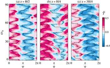
Fig. 1: Sidewall temperatures for  showing the ST oscillations. Time is normalised by the free-fall time-scale
  . The black lines indicate the maximum and minimum temperature (a) for midheight, exhibiting the typical signatures of a sloshing mode, and (b)–(c) for one and three quarter heights, where the minimum and maximum positions are out of phase with the midplane extrema, and the
  maximum and the
  minimum are in phase, indicating a torsional motion.
Download figure:
Standard image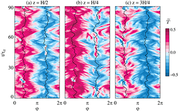
Fig. 2: Sidewall temperatures for  for the jump rope vortex (JRV), similar to fig. 1. The black lines indicate the LSC position according to eq. (7). The accordion-like sidewall signature of the JRV can be seen for all three vertical positions.
Download figure:
Standard imageQuasi-2D modes: sloshing and torsional (ST) oscillations
The torsional and sloshing motions found in cylinders with  are the best-studied LSC modes. They are sketched in fig. 3 in a decoupled view to highlight their principle behaviours. Both LSC modes can be described as quasi-2D planar movements: Torsional oscillations manifest through a periodic twist and counter-twist [7,48] whereas sloshing constitutes a horizontal back and forth displacement of the virtual LSC plane [8,29,32]. Brown and Ahlers described these modes in a unified stochastic framework [32,37–39], arguing that these oscillations are a manifestation of advected travelling waves along the LSC. Within this model, the sidewall provides a pressure gradient force that restores the slosh displacement and the torsional oscillations. Thus, these two LSC modes are coupled and the torsional mode cannot exist on its own without the slosh displacement. In fig. 1, sloshing is evident by its characteristic zigzag pattern at
  , i.e., the minimum and maximum of the temperature approach and recede from each other in an in-phase periodic motion. Torsional oscillations are revealed through the maximum and the minimum being out of phase in the lower and upper half of the cylinder at the same vertical positions, but with the maximum at
  and the minimum at
  being in phase. Since we are processing low-Pr numerical data with high azimuthal resolution, we can simply trace the minimum and maximum of the temperature. In laboratory experiments, the azimuthal resolution is typically limited and in medium-Pr fluids the thermal signal is weaker, thus, requiring either a sinusoidal fitting function extended to higher harmonics or the temperature extremum extraction (TEE) method to accurately locate the extrema [29,32]. The ST frequency can then be determined by evaluating the timeseries of the slosh and the torsion angle
  via
via


i.e., the angular difference between the maximum and minimum of the temperature at half height and the angular difference between the maximum at one-quarter and the minimum at three-quarter height, respectively. The  timeseries and corresponding spectra are presented in fig. 4(a) and (e). Both
  and
and  show a clean oscillation and accordingly a distinct, albeit relatively wide, spectral peak. The width of the peak is a result of the non-sinusoidal and "square-y" character of the ST oscillation that can be inferred from fig. 1. The black lines indicating the maximum and minimum temperatures show that the flow resides a finite time in each extremal position but the switch between these positions happens rapidly. The square waveform is also visible in the magnification of fig. 4(a), presented in fig. 4 in the SM, further supporting the notion that the width of the peak is thus a measure of the residence time.
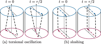
Fig. 3: Schematic of decoupled quasi-planar LSC modes at different stages of the oscillation period τ. At  and
and  the LSC plane is aligned with the vertical midplane. Adapted from Brown and Ahlers [32].
Download figure:
Standard image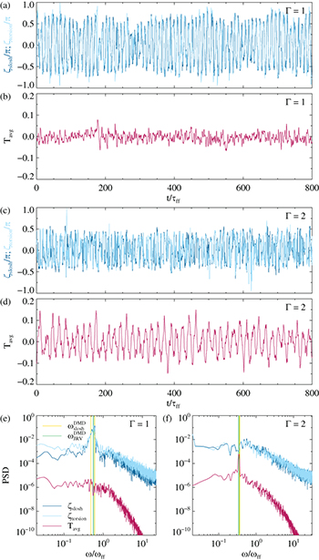
Fig. 4: (a), (c): Time series of the slosh and torsion angles according to eqs. (5), (6) for  and 2, respectively. (b), (d): time series of the mean temperature along the midheight cylinder circumference for
  and 2, respectively. (e), (f): corresponding spectra. The frequencies of two ST modes and two JRV modes identified via DMD are marked by the yellow and green vertical lines, respectively. The time series and frequency are normalised using the free-fall time
  and corresponding free-fall frequency
  .
.
Download figure:
Standard image3D mode: jump rope vortex (JRV)
The JRV is a fundamental 3D LSC mode that dominates for  and is best described as a twirling jump rope [30]. The interior 3D LSC's vortex core precesses in a jump rope-like motion in the direction opposite to that of the outer tank-filling LSC velocity flow field. In particular, this implies a substantial inherent vertical motion of the LSC in contrast to the ST modes. A single LSC exists for cylindrical cells with Γ up to approximately 2 [12,13]. For larger convection tanks, multiple circulations exist. In a
  Cartesian cell, the dynamics is also dominated by JRVs, in this case four separate vortices [31]. Pandey et al. [9] defined superstructures in RBC as coherent turbulent flow structure whose horizontal length-scale is greater than the height of the fluid layer. In that sense, the JRV is possibly the smallest superstructure.
In the Hovmöller diagram of fig. 2, the JRV reveals its presence through its distinct accordion pattern of strong temperature alternations along the circumference at all three heights  ,
,  and
and  . The temperature distribution is well described by an extended sinusoidal-fitting function [30],

where a and b give the relative amplitudes of the hot and cold sidewall signals, and  is the sidewall temperature averaged over the entire circumference. The angle
  denotes the symmetry plane of the LSC, which is marked by the black lines for both the cold downflow and the hot upflow in fig. 2. At half-height, the temperature oscillates in such a way that between two-thirds and one-third of the circumference are either below or above the arithmetic mean of the top and bottom temperature
  , which results in the quasi-periodic oscillations in the time series of Tavg
shown in fig. 4(d). The narrow, pronounced peak in the power spectrum in fig. 4(f) is characteristic of this sinusoidal signal.
, which results in the quasi-periodic oscillations in the time series of Tavg
shown in fig. 4(d). The narrow, pronounced peak in the power spectrum in fig. 4(f) is characteristic of this sinusoidal signal.
Applying identical analysis methods and comparing the results, reveals that  and
and  only exhibit regular oscillations and a spectral peak for
  , fig. 4(a), (e), but not for
  , fig. 4(c), (f). Vice versa, the Tavg
signal only possesses periodic oscillations for
, fig. 4(c), (f). Vice versa, the Tavg
signal only possesses periodic oscillations for  , fig. 4(d), (f), but not for
  , fig. 4(b), (e). Hence, based on these analyses, it appears that the 3D JRV mode is absent in the
  sample and, conversely, the quasi-2D ST modes appear to not exist in the
  sample.
Extracting the dominant LSC modes employing the dynamic mode decomposition (DMD)
We will now use the dynamic mode decomposition (DMD) [40,42] in its parallel [49], sparsity-promoting variant [50] to demonstrate that, in fact, all three modes are present in both cases and to gain further insights into their specific dynamics. DMD is particularly well-suited for this endeavour since it extracts the flow structures with a single frequency contents, such as the ST and JRV frequencies here, and sparsity promotion enables us to rank the modes according to their dynamical importance (see SM). DMD has successfully been applied in the context of turbulent RBC [41], thus, we only give a very short summary here.
We process full instantaneous real-valued flow fields from the goldfish DNS. For  , N = 1401 snapshots are used each 0.5 time units apart. For
  , N = 1301 snapshots are used, each 1.0 time units apart. This choice is largely dictated by memory requirements. Every snapshot is expressed as a column vector
  at a given time tk
with dimension
at a given time tk
with dimension  . The first N –1 snapshots are then cast in a matrix
  , and a singular value decomposition (SVD) is performed, i.e.,
  . The superscript H denotes the conjugate-transpose of a matrix, U represents the spatial structures, i.e., the POD modes, and W the temporal ones, the matrix Σ contains the singular values and determines the rank q of
  . The last N – 1 snapshots,
  are combined with the matrices U and W to calculate the optimal representation S of the linear mapping in the basis spanned by the POD modes between snapshots,
  . Finally, the complex eigenvectors
  and eigenvalues
  of S are used to calculate the dynamic modes as
  . The eigenvalues can be associated with the frequency and the decay rate of the DMD mode via the common logarithmic mapping,
  ,
,  , where
  is the time step between the snapshots. The approximate flow can be represented with

where ak are the complex amplitudes of the dynamic modes and k is the index of the included modes.
If we were to seek an optimal approximation of the entire flow using the dynamic modes  , the sparsity promoting algorithm [50] would retain many modes due to the strongly nonlinear and turbulent nature of the original system. E.g., for a maximum performance loss of 50%, 114 (422) dynamic modes (ignoring the complex-conjugate twin mode [41]) need to be kept for
  .
.
However, we can use the representation (8) to consider the temporal evolution of either a single mode or a small subset of modes. We employ the sparsity promoting algorithm to only retain eleven modes. The primary mode is the stationary mean (or base) flow, shown in fig. 5(a), (d). In both cases, the shape is that of an LSC. However, for  , the maximum and the minimum temperature are azimuthally off-centre within the warm upflow and the cold downflow, respectively, indicative of a tilted LSC plane. For
  , the maximum and minimum are approximately centred, this is best visible in the sidewall temperature signal at midheight shown in fig. 6(a), (d) and also in fig. 3 in the SM. This finding is in essential agreement with Brown and Ahlers [32], stating that the preferred orientation of the LSC is determined where it has the longest diameter. In addition, for both Γ, four low-frequency drifting modes are identified (not shown, see also fig. 1 in the SM).
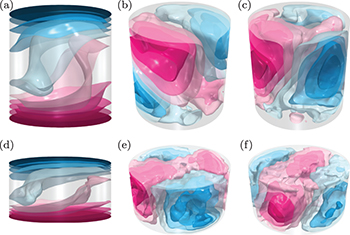
Fig. 5: Isosurfaces of the real part of the DMD temperature modes,  : (a)–(c)
  , (d)–(f)
  ; (a), (d): mean flow, (b), (e): superposition of two ST DMD modes, (c), (f): superposition of two JRV DMD modes.
Download figure:
Standard image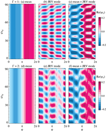
Fig. 6: Hovmöller diagram of the real part of the DMD temperature modes at midheight: (a)–(c)  , (d)–(f)
  ; (a), (d): mean flow, (b), (e): superposition of two JRV DMD modes, (c), (f): superposition of mean flow and JRV modes resulting in the characteristic accordion pattern. See fig. 5 in the SM for each JRV mode separately.
Download figure:
Standard imageFor  , all ten non-base flow modes represent some form of ST oscillations. The morphology of these modes is similar to the ones shown in fig. 5(b), a 4-roll state, which is symmetric with respect to the vertical and horizontal midplanes. Their oscillatory behaviour is slightly different, though. In particular, one of these 4-roll modes periodically completely collapses and then rebuilds itself with opposite sign, whereas another one achieves a similar sign-change by performing a circular motion, as shown in the supplementary movie
movie1.mp4
. When we superpose the mean flow with these two dominant 4-roll ST modes, we observe a characteristic zigzag slosh and torsional pattern at the sidewall, displayed in fig. 7(a)–(c), and similarly we see that this is the resulting motion in the supplementary movies
movie1.mp4
and
movie2.mp4
. The corresponding frequencies extracted via DMD are also marked in the spectra in fig. 4(e). The frequencies agree well with the ones obtained via the traditional method of determining the slosh and torsional angle. Moreover, the existence of several ST modes is in complete agreement with the broad peak observed in the spectrum of fig. 4(e); more modes are needed to reproduce a square wave. Whenever we considered more than eleven dynamic modes, we also identified modes that leave an accordion imprint on the sidewall. The 3D structure of two superposed modes is shown in fig. 5(c) and their thermal sidewall signal in fig. 6(c), (d) and supplementary movie
movie2.mp4
. Hence, this indicates that JRV modes also exist in a
, all ten non-base flow modes represent some form of ST oscillations. The morphology of these modes is similar to the ones shown in fig. 5(b), a 4-roll state, which is symmetric with respect to the vertical and horizontal midplanes. Their oscillatory behaviour is slightly different, though. In particular, one of these 4-roll modes periodically completely collapses and then rebuilds itself with opposite sign, whereas another one achieves a similar sign-change by performing a circular motion, as shown in the supplementary movie
movie1.mp4
. When we superpose the mean flow with these two dominant 4-roll ST modes, we observe a characteristic zigzag slosh and torsional pattern at the sidewall, displayed in fig. 7(a)–(c), and similarly we see that this is the resulting motion in the supplementary movies
movie1.mp4
and
movie2.mp4
. The corresponding frequencies extracted via DMD are also marked in the spectra in fig. 4(e). The frequencies agree well with the ones obtained via the traditional method of determining the slosh and torsional angle. Moreover, the existence of several ST modes is in complete agreement with the broad peak observed in the spectrum of fig. 4(e); more modes are needed to reproduce a square wave. Whenever we considered more than eleven dynamic modes, we also identified modes that leave an accordion imprint on the sidewall. The 3D structure of two superposed modes is shown in fig. 5(c) and their thermal sidewall signal in fig. 6(c), (d) and supplementary movie
movie2.mp4
. Hence, this indicates that JRV modes also exist in a  cylinder, but the stronger confinement suppresses their dynamical importance.
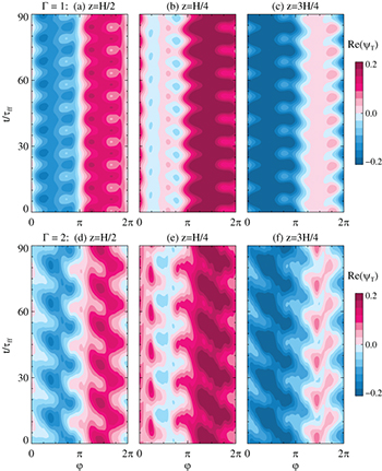
Fig. 7: Hovmöller diagram of the real part of the DMD temperature of a superposition of the mean flow and two ST modes resulting in the characteristic zigzag pattern. The upper panels (a)–(c) show the data for  , the lower panels (d)–(f) the data for
  ; (a), (d): at midheight
  , (b), (e):
  , (c), (f):
  . See fig. 6 in the SM for each ST mode separately.
Download figure:
Standard imageFor the  data, DMD reveals that two accordion modes are the most important dynamic modes. The 3D structure of a superposition of these two modes is shown in fig. 5(f) and the supplementary movie
movie3.mp4
. The corresponding Hovmöller diagram of the DMD modes with and without mean flow are shown in fig. 6(e)–(f). The remaining dominant modes are of ST type (less four drift modes). These
data, DMD reveals that two accordion modes are the most important dynamic modes. The 3D structure of a superposition of these two modes is shown in fig. 5(f) and the supplementary movie
movie3.mp4
. The corresponding Hovmöller diagram of the DMD modes with and without mean flow are shown in fig. 6(e)–(f). The remaining dominant modes are of ST type (less four drift modes). These  ST DMD modes exhibit a zigzag pattern that closely resembles the one found in
  , see fig. 7(d)–(f). However, there are also notable differences, as seen in the 3D visualisation of fig. 5(e) and the supplementary movie
movie4.mp4
. There is no clear 4-roll state, where two rolls are stacked on top of each other, instead the four rolls are all situated next to each other on the same level. Nonetheless, also these ST modes have an inherent symmetry with respect to the vertical midplane. Even a small deviation of the LSC from its upright position seems to induce a sloshing motion together with its associated torsional oscillation, which act to attempt to restore the LSC into a position that is aligned with the horizontal midplane.
, see fig. 7(d)–(f). However, there are also notable differences, as seen in the 3D visualisation of fig. 5(e) and the supplementary movie
movie4.mp4
. There is no clear 4-roll state, where two rolls are stacked on top of each other, instead the four rolls are all situated next to each other on the same level. Nonetheless, also these ST modes have an inherent symmetry with respect to the vertical midplane. Even a small deviation of the LSC from its upright position seems to induce a sloshing motion together with its associated torsional oscillation, which act to attempt to restore the LSC into a position that is aligned with the horizontal midplane.
Discussion
We now connect the DMD-based findings with the more traditional methods by separately analysing the two superposed ST and JRV modes. The slosh and torsional angles  ,
,  are shown in fig. 8(a), (c). The ST DMD modes exhibit regular oscillations in both the
  and in the
  geometry, thus providing further evidence that indeed in both aspect ratios a sloshing motion in combination with a torsional oscillation exists. The origin of the sloshing can be understood as the interaction or superposition of the LSC mean flow being tilted with respect to the horizontal midplane and a higher-order mode that is (anti)symmetric with respect to the horizontal and vertical midplanes. ST oscillations dominate the dynamics in
  cylindrical cells and also have some impact on the dynamics of
  cells. The midplane average temperature Tavg
is shown in fig. 8(b), (d). For the JRV modes, strong oscillations are visible, albeit with a much larger amplitude for
cells. The midplane average temperature Tavg
is shown in fig. 8(b), (d). For the JRV modes, strong oscillations are visible, albeit with a much larger amplitude for  compared to
  . Thus, the JRV mode is also present in both cases, indicating that it is indeed a very fundamental dynamic property of the LSC. Figure 8 further elucidates that the individual ST modes do not exhibit typical JRV characteristics, i.e., they do not show distinct regular oscillations in Tavg
. Similarly, the individual JRV modes do not exhibit ST characteristics, i.e., they do not show oscillations in
. Thus, the JRV mode is also present in both cases, indicating that it is indeed a very fundamental dynamic property of the LSC. Figure 8 further elucidates that the individual ST modes do not exhibit typical JRV characteristics, i.e., they do not show distinct regular oscillations in Tavg
. Similarly, the individual JRV modes do not exhibit ST characteristics, i.e., they do not show oscillations in  and
and  . The faint signatures of the respective other LSC mode type are detectable, because the JRV and ST frequencies are almost identical since both are set by the LSC path length and the free-fall velocity.
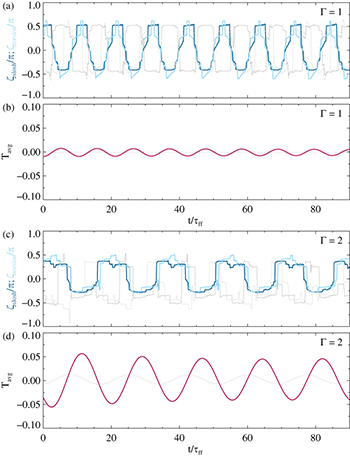
Fig. 8: Traditional analysis as shown in fig. 4(a)–(d) applied to the two selected ST and JRV DMD modes, respectively. (a), (b): analysis for  , (c), (d): analysis for
  . (a), (c): slosh and torsional angle
  ,
,  for the DMD ST (JRV) modes are shown in dark and light blue (grey), respectively. (b), (d): the average temperature around the midplane circumference Tavg
. The magenta line corresponds to the DMD JRV mode, showing a large amplitude oscillation. The grey line corresponds to the ST DMD mode, with a much smaller amplitude.
for the DMD ST (JRV) modes are shown in dark and light blue (grey), respectively. (b), (d): the average temperature around the midplane circumference Tavg
. The magenta line corresponds to the DMD JRV mode, showing a large amplitude oscillation. The grey line corresponds to the ST DMD mode, with a much smaller amplitude.
Download figure:
Standard imageTraditional analysis methods tend to identify either the JRV or the ST LSC mode. In contrast, DMD analysis reveals that both types of modes coexist with the JRV being dominant in higher Γ cylinders and the ST mode being dominant in lower Γ cylinders; figs. 4 and 8 demonstrate how to easily differentiate the JRV and the ST LSC mode using  ,
,  and Tavg
measurements.
and Tavg
measurements.
Acknowledgments
SH gratefully acknowledges funding by the EPSRC (grant EP/V047388/1) and JMA by the NSF Geophysics Program (EAR awards 1620649 and 1853196).
Data availability statement. All data that support the findings of this study are included within the article (and any supplementary files).
Footnotes
Contribution to the Focus Issue Turbulent Thermal Convection edited by Mahendra Verma and Jörg Schumacher.