


Abstract
We investigate the two-dimensional melting of deformable polymeric particles with multi-body interactions described by the Voronoi model. We report machine learning evidence for the existence of the intermediate hexatic phase in this system, and extract the critical exponent  for the divergence of the correlation length of the associated solid-hexatic phase transition. Moreover, we clarify the discontinuous nature of the hexatic-liquid phase transition in this system. These findings are achieved by directly analyzing system's spatial configurations with two generic machine learning approaches developed in this work, dubbed "scanning-probe" via which the possible existence of intermediate phases can be efficiently detected, and "information-concealing" via which the critical scaling of the correlation length in the vicinity of generic continuous phase transition can be extracted. Our work provides new physical insights into the fundamental nature of the two-dimensional melting of deformable particles, and establishes a new type of generic toolbox to investigate fundamental properties of phase transitions in various complex systems.
Export citation and abstract BibTeX RIS
Introduction
The nature of two-dimensional (2D) melting [1] is delicate and can show non-trivial dependence on several properties of the specific systems, e.g., softness [2,3], activity [4–8], density [9], potential [10–14], pinning of particles [15], shape of particles [16,17], topological constraints [18], etc. Three different types of 2D melting scenarios, namely, the one-step melting scenario [19], the hard-disk–like scenario [20–22], and the Kosterlitz-Thouless-Halperin-Nelson-Young scenario [23–26] have been identified. However, some questions are still left open. The most important ones include the existence of the intermediate hexatic phase and the fundamental nature of its associated phase transitions.
To solve these open questions, one crucial step is to identify different phases in the relevant systems. This is usually done via investigating the spatial decay of correlation functions of the translational order and the bond-orientational order, combined with the unbinding behavior of dislocations and disclinations [23–26]. More specifically, it is suggested that the solid-hexatic phase transition is associated with the disappearance of the quasi-long range translational order and the increasing number of dislocations [2], and that the hexatic-liquid phase transition is associated with the disappearance of the long range bond-orientational order and the dissociation of the dislocation into disclinations [2]. However, a firm confirmation within this approach is still difficult, partially due to the possibly enormous value of the hexatic correlation length [12] and also the fact that other complicated defects, such as vacancies and grain boundaries, might appear near the phase transitions [27–29]. Noticing that machine learning techniques have emerged in recent years as an efficient tool to investigate various problems on phase transitions [30–48], this thus raises the intriguing opportunity to develop new tools based on these powerful techniques to reveal new physical insights into these open questions, in particular, the ones concerning the existence of the intermediate hexatic phase and the fundamental nature of its associated phase transitions, especially the possible critical scaling behavior.
In this work, we address these questions for the 2D melting of deformable polymeric particles with multi-body interactions described by the Voronoi model [2,49–54]. To this end, we develop two generic neural network-based machine learning approaches dubbed "scanning-probe" (cf. fig. 1(a)) and "information-concealing" (cf. fig. 2(a)) to directly analyze a large number of system's spatial configurations that are generated by Brownian dynamics simulations, and find the following.
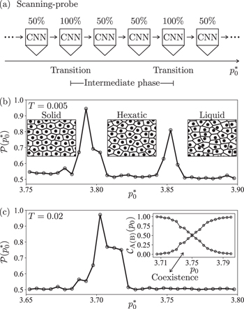
Fig. 1: (a) Schematic illustration of "scanning-probe" machine learning. The "phase-transition-probe" is realized by a deep CNN that is able to give the signal  on how likely there is a phase transition in a narrow parameter interval
 ![$[p_{0}^{*}-\Delta p_{0},p_{0}^{*}+\Delta p_{0}]$](https://content.cld.iop.org/journals/0295-5075/136/4/48002/revision3/epl21100703ieqn3.gif) , where
, where  indicates the existence of a possible transition, with
  being the suspected phase transition point and
  being the resolution of the probe. (b) Identification of the intermediate hexatic phase at a low temperature
  . The classification accuracy
  associated with the "phase-transition-probe" manifests two pronounced peaks that signify two phase transitions and hence three distinct phases, with the intermediate one corresponding to the hexatic phase. And these double peaks correspond to the solid-hexatic phase transition point
  and the hexatic-liquid phase transition point
  , respectively. Inset: typical samples of the data in the solid phase (left), the hexatic phase (middle), and the liquid phase (right). (c) Identification of the intermediate hexatic phase at a relatively high temperature
  . The classification accuracy
  associated with "phase-transition-probe" manifests only a single peak in this case, and this peak corresponds to the solid-hexatic phase transition point with
  . Inset: the auxiliary machine learning to resolve the hexatic-liquid phase coexistence. Two average confidence values
  of the deep CNN show big differences around
  in the vicinities of both ends of the parameter interval
 ![$[3.705,3.800]$](https://content.cld.iop.org/journals/0295-5075/136/4/48002/revision3/epl21100703ieqn16.gif) for p0, clearly indicating that there exist two distinct phases around
for p0, clearly indicating that there exist two distinct phases around  and
and  , i.e., the hexatic phase and the liquid phase. The parameter region around the intersection point is expected to correspond to a phase coexistence region of these two phases, and the upper bound for the hexatic phase region can be estimated by this point with
  . See text for more details.
Download figure:
Standard imagei) Machine learning evidence for the existence of the intermediate hexatic phase (cf. fig. 1). At the low temperature, when the so-called target shape index of the system increases, the classification accuracy (cf. eq. (3)) associated with the "phase-transition-probe" manifests two pronounced peaks that signify two phase transitions and hence three distinct phases, with the intermediate one corresponding to the hexatic phase (cf. fig. 1(b)). At the relatively high temperature, the single peak behavior of the classification accuracy of the "phase-transition-probe", combined with the phase coexistence region identified by an auxiliary machine learning, still indicates the existence of three distinct phases with the intermediate one corresponding to the hexatic phase (cf. fig. 1(c)). The identified phase coexistence region also clarifies the discontinuous nature of the hexatic-liquid phase transition in this system.
ii) The continuous solid-hexatic phase transition manifests a critical scaling behavior with the critical exponent  for the divergence of the correlation length (cf. fig. 2). We observe that at different temperatures, the good data collapse is achieved for the average outputs of the convolutional neural network (CNN) employed in "information-concealing" machine learning as a function of the reduced target shape index when it is rescaled with the critical exponent
  (cf. figs. 2(c), (e)) with respect to the linear size l of the system after "concealing", clearly manifesting the critical scaling behavior of the correlation length in the vicinity of the continuous solid-hexatic phase transition.
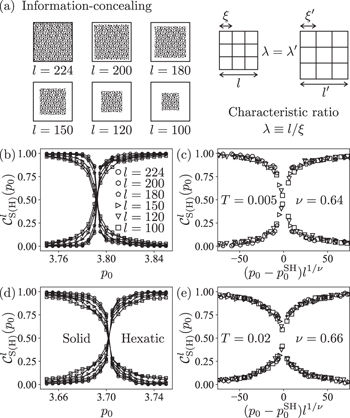
Fig. 2: (a) Schematic illustration of "information-concealing" machine learning. The peripheries of the samples in the original dataset are deliberately concealed to generate a series of datasets with reduced effective areas characterized by the effective length scale l for their samples. The ratio between l and the system correlation length  , i.e.,
  , determines the information content of the system that can be utilized by the CNN to perform the classification task. For instance, a small sample with linear size l and a correlation length
  is expected to contain the same amount of information for the CNN as a larger sample with linear size
  and a larger correlation length
  if
if  . This indicates that the critical exponent ν for the divergence of the correlation length can be extracted via the data collapse behavior of the average confidence values that performs the classification task with respect to datasets with samples of effective length scale l. (b) Average confidence values of the CNN to classify the hexatic phase from the solid phase using datasets with different fixed l at the low temperature
  . (c) The good data collapse is achieved for the average confidence values in (b) as a function of
  with the critical exponent
  . (d) Average confidence values of the CNN to classify the hexatic phase from the solid phase using datasets with different fixed l at the relatively high temperature
  . (e) The good data collapse is achieved for the average confidence values in (d) as a function of
  with the critical exponent
  . See text for more details.
Download figure:
Standard imageSystem and model
The system under study consists of N deformable polymeric particles with multi-body interactions [2], whose elastic energy E is modeled according to the Voronoi description [49–54],

where Ai
and Pi
are the cross-sectional area and the perimeter of the i-th particle, A0 and P0 are the preferred particle area and perimeter, KA
and KP
represent the area and perimeter stiffness moduli, respectively. This Voronoi model originates from the investigations of the confluent cells in biological tissues, where the first term in eq. (1) models the cell incompressibility and the monolayer's resistance to height fluctuations, and the second term arises from the active contractility of the actomyosin subcellular cortex and the effective cell membrane tension due to the cell-cell adhesion and cortical tension. The effective dimensionless target shape index  is an important parameter that controls the elastic behavior of these deformable particles. The elastic energy in eq. (1) leads to a mechanical interaction force on the i-th particle by
  , which is a multi-body interaction force that cannot be expressed as a sum of pairwise force between the i-th particle and its neighbors [49–54]. To simulate the dynamics in this system, each particle undergoes overdamped Brownian motion at a given temperature T. Thus, the dynamics of the deformable particles in the overdamped limit follows the Langevin equation [49–54]

where μ is the mobility, kB
is the Boltzmann constant, and  are Gaussian white noises with zero mean and unit variance. Equations (1), (2) can be rewritten in the dimensionless forms by introducing the characteristic length
  and time
  . The parameters in the dimensionless forms can be rewritten as
  and
and  . We shall omit the hat for all quantities occurring in the above equations from now on and use only the dimensionless variables.
From the expression for the elastic energy in eq. (1), we can see that at fixed temperature T, the system softens when the target shape index p0 increases. Therefore, one naturally expects a solid phase with small p0, and a liquid phase with large p0. With an intermediate p0, one so-called hexatic phase could possibly emerge as an intermediate phase between the solid and the liquid phases. Recent investigations [2–4,49–54] have shown numerical evidence that supports the existence of the intermediate hexatic phase in this system from properties of the translational correlation function, the bond-orientational correlation function, and different types of topological defects such as dislocations and disclinations. However, potential limitations of the existing evidence were also reported, for instance, the exponent of the asymptotic power law decay of the correlation functions can be difficult to extract due to the limited system size employed in the study [5,12], and the relevant types of topological defects that drive the phase transition associated with the intermediate hexatic phase are still under debate [27–29]. In this regard, a type of approaches that directly analyzes the system's spatial configurations with as few build-in empirical assumptions as possible is highly desirable to provide new physical insights into the questions concerning the existence of the intermediate hexatic phase and the fundamental nature of its associated phase transitions in this system. Indeed, as we shall see in the following sections, such a type of approaches can be developed by utilizing the modern machine learning techniques [55,56].
Here in this work, we focus on the case with  , and set the particle number N = 3960 (cf. the Supplementary Material
Supplementarymaterial.pdf (SM)
1
for an investigation on the finite size effect, which shows that it does not impose strong influences on the major results presented in the following). The configurations to be directly processed by the machine learning approaches developed in the following are obtained by Brownian dynamics simulations of the system in a 2D rectangular space with aspect ratio
, and set the particle number N = 3960 (cf. the Supplementary Material
Supplementarymaterial.pdf (SM)
1
for an investigation on the finite size effect, which shows that it does not impose strong influences on the major results presented in the following). The configurations to be directly processed by the machine learning approaches developed in the following are obtained by Brownian dynamics simulations of the system in a 2D rectangular space with aspect ratio  and periodic boundary condition imposed. The initial configuration is chosen to be a perfect hexagonal lattice. With different fixed values for (T, p0), we typically generate
  of system's spatial configurations in the steady state, and transform these configurations into images according to the Voronoi tessellation [49–54] (see the SM for more technical details on the data generation).
Intermediate hexatic phase identified via "scanning-probe"
To identify the intermediate hexatic phase, we need a high-resolution machine learning approach to efficiently detect multiple phase transitions triggered by tuning a single system parameter, in contrast to most of the well-established machine learning approaches that are experts in searching for a single phase transition in a large parameter region [31,32]. Here, we develop a generic machine learning approach dubbed "scanning-probe", in which the key workhorse is a "phase-transition-probe" that is able to give the signal on how likely there is a phase transition in a narrow parameter interval ![$[p_{0}^{*}-\Delta p_{0},p_{0}^{*}+\Delta p_{0}]$](https://content.cld.iop.org/journals/0295-5075/136/4/48002/revision3/epl21100703ieqn44.gif) with
with  being the suspected phase transition point and
  being the resolution of the probe. Since the hexatic phase can be far from obvious in the real space (cf. insets of fig. 1(b)), the "scanning-probe" approach can be realized by a deep CNN that has strong feature extraction ability, where the network is trained as a binary classifier by using the data associated with the two boundaries of the interval. More specifically, we label all the samples with
  as "phase A" and the ones with
  as "phase B", and the probe's signal concerning the phase transition is given by the classification accuracy
  in the testing process of the trained CNN, whose explicit form reads

with M being the number of test samples associated with each p0 and  being the number of test samples that have been identified successfully as phase A (B) by the CNN. Here, the CNN gives two outputs
  , where
  can be regarded as a classification confidence value
 ![$\in[0,1]$](https://content.cld.iop.org/journals/0295-5075/136/4/48002/revision3/epl21100703ieqn53.gif) of how likely the sample is in phase A (B). For a sample fed to the CNN, it is identified as phase A if
of how likely the sample is in phase A (B). For a sample fed to the CNN, it is identified as phase A if  or phase B if
  . As one can naturally expect if the two groups of data belong to the same phase physically, there should be no essential difference between each other, hence the CNN can only learn to trivially identify all the samples as the same phase. This leads to either
  or
or  , i.e.,
  , which is equivalent to a random guess. On the contrary, if there indeed exists a phase transition in the interval
 ![$[p_{0}^{*}-\Delta p_{0},p_{0}^{*}+\Delta p_{0}]$](https://content.cld.iop.org/journals/0295-5075/136/4/48002/revision3/epl21100703ieqn59.gif) , the two groups of data can naturally manifest certain distinct differences from each other that can be learned by the CNN, hence the classification accuracy is expected to be very high, i.e.,
, the two groups of data can naturally manifest certain distinct differences from each other that can be learned by the CNN, hence the classification accuracy is expected to be very high, i.e.,  , which can be used as a clear signal for the phase transition point (see the SM for more technical details on the network training).
Via making a scanning with the "phase-transition-probe" over the complete parameter region of interests, possible phase transitions in it can be detected. Since each probing involves only two groups of data that correspond to  and
and  , the computational cost of the "scanning-probe" approach scales linearly with respect to the number of the suspected parameter points in the complete parameter region. This is in contrast to the machine learning approaches that employ all the data, e.g., the confusion scheme [32], whose computational cost scales quadratically with respect to the number of the suspected parameter points.
We first consider a nearly zero-temperature case at  . As we can see from fig. 1(b), the
  dependence of
  manifests two pronounced peaks, indicating that there should exist three distinct phases in this system. From the expression of the system's elastic energy in eq. (1), we know that the system becomes harder as the target shape index p0 becomes smaller, hence the system with a very small target shape index p0 is expected to be in the solid phase. Combining this physical understanding with the behavior that
  on the left side of the left peak in fig. 1(b), which manifests that the system's spatial configurations associated with the small interval
 ![$[p_{0}^{*}-\Delta p_{0},p_{0}^{*}+\Delta p_{0}]$](https://content.cld.iop.org/journals/0295-5075/136/4/48002/revision3/epl21100703ieqn67.gif) show no significant difference among them, we can conclude that the system is solid if p0 is smaller than the target shape index value corresponding to the left peak. In contrast, the system with a very large p0 should be in the liquid phase, since the increase of p0 favors less compact shapes and thus a reduction in the number of sides of the Voronoi tessellation [2–4,49–54]. Combining with the fact that
show no significant difference among them, we can conclude that the system is solid if p0 is smaller than the target shape index value corresponding to the left peak. In contrast, the system with a very large p0 should be in the liquid phase, since the increase of p0 favors less compact shapes and thus a reduction in the number of sides of the Voronoi tessellation [2–4,49–54]. Combining with the fact that  on the right side of the right peak in fig. 1(b), we can conclude that the system is liquid if p0 is larger than the target shape index value corresponding to the right peak. In this regard, one can naturally arrive at a further conclusion that an intermediate phase exists between the two peaks, which is neither the solid phase nor the liquid phase, and is expected to be the intermediate hexatic phase that emerges between the solid and the liquid phases in 2D systems. Consequently, the left peak in fig. 1(b) corresponds to the solid-hexatic phase transition point with
  , while the right one corresponds to the hexatic-liquid phase transition point with
  , which is consistent with the phase transition points
  and
and  at
at  identified via conventional approaches [2], providing strong machine learning evidence for the existence of the intermediate hexatic phase.
We further investigate a relatively high temperature case at  . In this case, the deep CNN detects only a single peak, as shown in fig. 1(c). This seems to imply that there exist only two phases at this temperature. However, we note that the signal of the "phase-transition-probe" (cf. eq. (3)) is associated with a narrow parameter interval
 ![$[p_{0}^{*}-\Delta p_{0},p_{0}^{*}+\Delta p_{0}]$](https://content.cld.iop.org/journals/0295-5075/136/4/48002/revision3/epl21100703ieqn75.gif) . If there exists a strong phase coexistence in the certain parameter region, as ubiquitous in the vicinities of the first-order phase transitions, the probe indeed can also give the signal
. If there exists a strong phase coexistence in the certain parameter region, as ubiquitous in the vicinities of the first-order phase transitions, the probe indeed can also give the signal  in this parameter region despite possible first-order phase transitions could exists. Therefore, the single peak in fig. 1(c) might also indicate that there exists a relatively large phase coexistence parameter region on its right. This motivates us to perform an auxiliary machine learning, where we train the CNN using the data associated with two parameter points that are well separated from each other. More specifically, we use the data with
  and
and  , and label all the samples associated with the former as "phase A" and the latter as "phase B". We then test the average confidence values
  of the trained CNN for
  , where
  and 〈·〉 denotes the average over M test samples associated with each p0. As we can see from the inset of fig. 1(c), the average outputs
  , i.e., the average classification confidence values associated with phase A and phase B, show big differences around
  in the vicinities of both ends of the parameter interval
 ![$[3.705,3.800]$](https://content.cld.iop.org/journals/0295-5075/136/4/48002/revision3/epl21100703ieqn84.gif) for p0. This clearly indicates that there indeed exist two distinct phases around
for p0. This clearly indicates that there indeed exist two distinct phases around  and
and  , and thus the parameter region around the intersection point in the inset of fig. 1(c) is expected to correspond to a phase coexistence region. From the expression of the system's elastic energy in eq. (1), we know that the systems with the small p0 on the left side of the peak are in the solid phase. While the intersection point in the inset of fig. 1(c) appears far right of the peak, so the phase coexistence around the intersection point is not relevant to the solid phase, but should be a coexistence between the hexatic and the liquid phases. Therefore, we can conclude that the peak in fig. 1(c) corresponds to the solid-hexatic phase transition point
  , which is also consistent with the phase transition point
  at
at  identified via conventional approaches [2], and that the intersection point in the inset of fig. 1(c) should correspond to an upper bound of the hexatic phase region with
  . Moreover, the existence of this relatively large phase coexistence region naturally leads to the conclusion that the hexatic-liquid phase transition in this system is discontinuous.
Critical scaling extracted via "information-concealing"
So far, we have identified the intermediate hexatic phase and clarified the discontinuous nature of the hexatic-liquid phase transition. One fundamental question still left is the critical scaling of the solid-hexatic phase transition. To address this question, we develop a generic machine learning approach dubbed "information-concealing" that is able to extract the critical scaling of the correlation length in the vicinity of a generic continuous phase transition.
This approach is based on the natural expectation that for a CNN employed to perform a classification task in a translational invariant way, its outputs, i.e., the classification confidence values, shall be dominated by the features whose characteristic length scales are given by the correlation length ξ of the system. This thus indicates that the content of the effective information of each sample of the data, which the CNN can utilize to perform the classification task, is determined by a characteristic ratio  with l being the length scale of the effective area of the sample (cf. fig. 2(a)). Consequently, for two different samples, as long as their characteristic ratios λ are the same, their corresponding average confidence values of the CNN are expected to be the same, too. This directly indicates that for a generic continuous phase transition triggered by tuning a system parameter g across its critical value gc
, the average confidence values as a function of the rescaled system parameter
with l being the length scale of the effective area of the sample (cf. fig. 2(a)). Consequently, for two different samples, as long as their characteristic ratios λ are the same, their corresponding average confidence values of the CNN are expected to be the same, too. This directly indicates that for a generic continuous phase transition triggered by tuning a system parameter g across its critical value gc
, the average confidence values as a function of the rescaled system parameter  with different fixed l should collapse to the same universal function near the phase transition, since the correlation length ξ generically manifests the power law behavior
  in the vicinity of the continuous phase transition with ν being the critical exponent for the divergence of the correlation length. Therefore, the critical exponent ν can be determined according to the data collapse behavior of the average confidence values as a function of the rescaled system parameter
  with different fixed l.
To implement the "information-concealing" approach, the information of the samples in the original dataset are deliberately concealed to generate a series of datasets with reduced effective areas for their samples. Each of these samples with reduced effective areas is obtained by randomly choosing an area of  pixels from the original images and conceal its periphery with the white color (cf. fig. 2(a)). The critical scaling of the correlation length ξ in the vicinity of the phase transition under consideration is then straightforwardly obtained by investigating the data collapse behavior of the average confidence values as a function of the rescaled system parameter
  with different fixed l (see the SM for more technical details). A benchmark of this approach is presented in the SM, where a good estimation of the critical exponent
  (exact value
  [57]) for the ferromagnetic-paramagnetic transition of the 2D Ising model is obtained.
We directly apply this "information-concealing" approach to reveal the critical scaling of the solid-hexatic phase transition in deformable particles with the CNN employed to perform the classification tasks. More specifically, we first perform "concealing" with a choice of effective length scale l to generate the corresponding dataset. Then, this complete dataset is used to train the CNN to perform the classification between the solid and the hexatic phases. After training, the CNN is able to output the classification confidence values  concerning the samples with corresponding target shape index p0, i.e., establish a map between the average confidence values
  , where
  , and the target shape index p0, from which the phase transition point
  is identified by the p0 where
  . We repeat this process with a series of different choices of the effective length scale
  , and get the corresponding
  and
and  . Figure 2(b) shows the dependence of the average confidence values on p0 with different fixed l at the low temperature
  , where the behaviors differ with respect to the target shape index p0. However,
  indeed shows the same dependence on its rescaled target shape index
  with
with  , as shown in fig. 2(c), indicating that the critical exponent ν for the divergence of the correlation length of the solid-hexatic phase transition assumes the value
  . We further perform the similar investigation at the relatively high temperature
  , the key results of which are shown in figs. 2(d), (e), where we notice that the good data collapse for the average confidence values is observed for
  . This is consistent with the value of the critical exponent obtained at
  , indicating that the critical scaling of the correlation length ξ in the vicinity of the solid-hexatic phase transition is given by the power law
  with
with  .
.
Finally, we remark that both "scanning-probe" and "information-concealing" machine learning involve no special design of the CNN structure. A widely used standard 18-layer residual neural network [58] is employed to perform the analysis as shown in fig. 1 and fig. 2 in the main text. In the SM, we present the same analysis employing another type of deep CNN called "GoogLeNet" [59], which gives the same results as the ones obtained by the residual neural network. This clearly shows the CNN structure independence of the two approaches developed in this work, which is indispensable for the reliability of the physical results they predict. Moreover, this also indicates the wide generic applicability of these approaches in investigating other relevant complex systems.
Conclusion and outlook
By directly analyzing system's spatial configurations via "scanning-probe" and "information-concealing" machine learning developed in this work, we provide machine learning evidence for the existence of the intermediate hexatic phase in 2D interacting deformable polymeric particles, and obtained the critical scaling behavior of the solid-hexatic phase transition, where the divergence of the correlation length is determined by a power law with the critical exponent  . Since these two machine learning approaches involve no special design for the CNN employed, they can be readily employed as a new generic toolbox to investigate the existence of the intermediate phase and the possible critical scaling behavior in various complex systems. For instance, we believe that our work will stimulate further efforts in revealing the critical scaling behavior of the solid-hexatic phase transition in nonequilibrium complex systems, e.g., in self-propelled biological tissues, via these new approaches. Moreover, noticing that the deep CNNs employed here are in general quite powerful in pattern recognition, we also expect that our machine learning approaches can be applied to investigate the physics associated with 2D microphase separations [62–65] in various complex systems.
Acknowledgments
We thank Jiajian Li for useful discussions. This work was supported by NSFC (Grant No. 11874017 and No. 12075090), GDSTC (Grant No. 2018A030313853 and No. 2017A030313029), GDUPS (2016), Major Basic Research Project of Guangdong Province (Grant No. 2017KZDXM024), Science and Technology Program of Guangzhou (Grant No. 2019050001), and START grant of South China Normal University.
Data availability statement: The data that support the findings of this study are available upon reasonable request from the authors.
Footnotes
- 1
See the SM, which includes refs. [31,41,55–61], for i) technical information about the data generation and the network training, ii) a benchmark of the "information-concealing" approach, iii) results that show the CNN structure independence of both approaches developed in this work, and iv) investigations on influences of the finite size effect and the number of samples in the dataset.