


Abstract
This paper deals with vortices in Maxwell-Chern-Simons models with nonminimal coupling. We introduce constraints between the functions that govern the model and find the conditions to minimize the energy. In this direction, a set of first-order equations with novel features are obtained, allowing us to smoothly modify the slope of the function that drives the scalar field in the rotationally symmetric configurations. The results show that, under specific conditions, the solutions may attain an inflection point outside the origin, while the energy density and the electric and magnetic fields get a ringlike profile. We also introduce a procedure to get multiring vortex configurations whose associated solutions engender several inflection points.
Export citation and abstract BibTeX RIS
Vortices in relativistic models started being investigated by Nielsen and Olesen in ref. [1]. They arise under the action of a complex scalar field minimally coupled to a gauge field under a U(1) symmetry. In this model, these objects are electrically neutral and exhibit a magnetic flux which is quantized by its vorticity. They are governed by equations of motion of second order with couplings between the fields. To get first-order equations, one may follow the Bogomol'nyi procedure and find the conditions for which the energy is minimized [2]. A manner to introduce the electric charge is by exchanging the Maxwell term with the Chern-Simons one [3,4], which also supports a first-order formalism that leads to minimum energy solutions. When dealing with Maxwell-Chern-Simons models [5–9], however, one must include a neutral field to perform the Bogomol'nyi procedure.
Instead of considering the addition of a neutral field, one may consider a nonminimal coupling between the fields, which includes an anomalous magnetic moment in the covariant derivative in the space of the fields [10–13]. Interestingly, in this situation, there are two routes to perform the Bogomol'nyi procedure. Depending on the constraints imposed to the model, one may get different sets of first-order equations that may lead to vortex configurations with distinct behavior [14], including the possibility of having magnetic flux inversion, which appears in the investigation of two-component superconductors [15], and also in Lorentz-violating models [16].
For rotationally symmetric solutions, the minimum energy configurations in models with minimal coupling always require the first-order equation which governs the scalar field to only support monotonic solutions [17]. However, the presence of the anomalous magnetic moment in the nonminimal coupling may change this feature. In this paper, we investigate the possibility of modifying the slope of the function associated to the scalar field in vortex configurations in models with nonminimal coupling, leading to inflection points in the solutions in the extreme case.
We consider the action of a complex scalar field φ nonminimally coupled to a gauge field  through a local U(1) symmetry in (2, 1) spacetime dimensions, with Lagrangian density

In this expression,  , where
  is the dual of the electromagnetic tensor
  . Notice that the function
  controls the modification in the anomalous magnetic moment, which brings the nonminimal coupling to light. The case
  recovers the minimal coupling. The function
  modifies the electric permittivity and the magnetic permeability of the system and
  drives the dynamical term of the scalar field and can be seen as a conformal factor for a metric in the space of the scalar field. The study of vortices in models of the Maxwell or Chern-Simons type with the inclusion of these functions was previously considered in refs. [18–20]. Here, we take μ and M in the above Maxwell-Chern-Simons model such that one may get a first-order formalism. Also, we use natural units
  . This model was studied in ref. [14], where we have thoroughly investigated its properties. So, we follow its lines to get the general equations for our paper. The equations of motion are


 and the subscripts denotes partial derivatives, i.e.,
  ,
,  ,
,  and
and  . The energy density is calculated standardly; it is given by
in which  is the covariant derivative associated to the usual minimal coupling. Also, the components of the electric field
  are defined by
  , and the magnetic field is
  . First-order formalism for Maxwell-Chern-Simons models with nonminimal coupling was developed in ref. [14]. So, we follow its lines and take

In this case, the equation of motion (2b) is solved by  , which allows us to relate the charge density with the magnetic field, as
  . Since the magnetic flux is given by
  , the charge is given by
  .
.
We have found that the novel configurations that we are interested in appear for

So, the form of  drives
  as in the above equation, and also
  , as one can see from eq. (4). This choice is a particular case of a more general model that was investigated in ref. [14]. However, as we shall see, it brings novel configurations to light. For convenience, we introduce the functions
  and
and  to rewrite the fields in the form
  and
and  , where
  , with
  . By doing so, the expression
  reads
reads

One can combine the above expression with the energy density in eq. (3) to get

in which we have used the notation  and
and  . To combine the last two terms of the above expression in a single derivative, we take the potential in the form

In this expression, v arises as an integration constant and is a parameter involved in the symmetry breaking of the system. At this point, we see that the model is exclusively specified by the function  . This procedure leads us to the energy
where

Notice this function does not depend on the function  . We integrate the last term in eq. (9) by parts to get
in which  denotes
  evaluated at r → ∞. The integrand of the last term is zero everywhere except at the points in which
  , because one has
  , where
  represents the zeros of φ (see ref. [13]). From the above equation, one can see that the energy is bounded,

Thus, the configurations with minimum energy arise if the following first-order equations are satisfied:


 which depends only on the magnetic flux and on the function
  at r → ∞. These equations can be combined with eq. (6) to lead us to
We remark that the potential must have the form in eq. (8). We have checked that eqs. (13) and (14) with the potential (8) satisfy the equations of motion (2).
To investigate rotationally symmetric vortices with topological character, we consider static fields and the usual ansatz  , where
  is the vorticity. Notice that the fields are now driven by three functions: g(r), h(r) and a(r). They must satisfy the boundary conditions
  ,
,  ,
,  ,
,  ,
,  ,
,  . The electric and magnetic fields take the form

so the magnetic flux is  . The first-order equations (13) read


At the origin, since  , we have
  . On the other hand, asymptotically, we must have
  , as
, as  . The equations with upper and lower sign are related by taking
  and
and  . We only work with the equations for the upper signs. Since we are interested to find novel behavior in the internal structure of the solutions, we consider M(v) to be finite and non-null, in order to avoid modifications in its tail.
The energy density (3) for the solutions of the first-order equations (16) is given by

This expression allows us to get the boundary condition for a(r). Since the energy is  , we impose
  to get finite energy solutions. In this situation, the magnetic flux below eq. (15) becomes
  and the energy in eq. (12) takes the form
  . Notice that these physical quantities are independent of the function
  and, also, quantized by the vorticity n.
We highlight that eq. (16a) is different from the corresponding equation that appears in the study of vortices models with minimal coupling,  , which only leads to a monotonic profile for g(r) in the study of topological solutions, even for generalized models [17]. Here, M(g) appears in the denominator in the right-hand side of the first-order equations (16) and the energy density (18). So, this function can be used to generate zeroes in
  , in the magnetic field and in the energy density, such that both the solutions g(r) and a(r) engender plateaux at these points. One has to be careful, though, as the solutions must obey the boundary conditions previously stated above eq. (15). To illustrate this novel feature, we take

where  and 0 < w < v are the parameters that control the model. The above function is positive where the solution exists, in the interval
  . We then have
  for
for  and
and  for
for  . This implies that the function
  defined by eq. (4) is negative for
  and becomes positive for
  . We remark that, although
  has a negative part, the energy density is positive; see eq. (18). From eq. (5), one can see that
  leads to
  and
and  , so the anomalous magnetic moment vanishes and the pure Chern-Simons model [3,4] is recovered. As λ increases, the function M gets a larger and larger value at the point
  , defined by
  , so we expect the derivative of the solutions to become smaller and smaller at this point. In the limit λ → ∞, one has

which is divergent at  . The potential in eq. (8) takes the form

which, in the limit λ → ∞, becomes

In fig. 1, we display the potential (21) for  ,
,  , and several values of λ, including
  and the infinite limit given in the above equation. One can see that the behavior of the potential changes significantly with λ at
  , for which
  . Starting with
  , we can see that this point determines a maximum. As λ increases, its height goes down until
  . For
. For  , this point becomes a local minimum of the potential. In the limit λ → ∞, we have
  , so the potential gets a global minimum at this point.

Fig. 1: The potential  in eq. (21) for
  ,
,  and
and  and the limit λ → ∞. The dotted line represents the case
  and the dashed one stands for the limit λ → ∞, described by eq. (22).
Download figure:
Standard imageFor a general λ, the first-order equations (16) read


 , we take
  and
and  , where
  , in (24). Expanding up to the lowest order in gw
and aw
, we get
, in (24). Expanding up to the lowest order in gw
and aw
, we get 
The above expression allows us to see that the function g(r) gets an inflection point at  in the case λ → ∞. This also occurs with a(r) and h(r); since the analysis is similar, we omit it here.
In fig. 2, we display the solutions for  ,
,  and several values of λ. The point
  is an inflection point of the solutions in the limit λ → ∞, such that
  ,
,  and
and  . As far as we know, the presence of this feature in g(r) is new in the study of relativistic vortices.

Fig. 2: The solutions g(r) (left), a(r) (middle) associated to eqs. (23), and h(r) (right) in eq. (17) for  ,
,  and
and  and the limit λ → ∞. The bottom panels shows the behavior of these solutions near the point
  . The dotted lines stand for
  and the dashed ones represent the limit λ → ∞.
Download figure:
Standard imageThe energy density (18) takes the form
whose limit for λ → ∞ is

Notice the presence of a global factor that vanishes at the point  , for which
  , in the above expression. This gives rise to a ring in the energy density whose location depends on w. In fig. 3 we plot the energy density (26) and the electric and magnetic fields in eq. (15) associated to the solutions of eqs. (23) for several values of λ, including the limit λ → ∞. We can see that the parameter λ modifies the inner behavior of the structure, leading to a set of zeroes outside the origin in these physical quantities. To better illustrate this feature, we display them in the plane in fig. 4. It shows how the parameter λ digs the structure to form a ring. In this sense, our model introduces a method to smoothly modify the slope of the solutions while the associated energy density and electric and magnetic fields go from a disk to a ringlike structure.
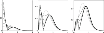
Fig. 3: The energy density in eq. (26) (left) and the electric (middle) and magnetic (right) fields in eq. (15) displayed in terms of the spatial coordinate r, for  ,
,  and
and  and the limit λ → ∞. The dotted lines stand for
  and the dashed ones represent the limit λ → ∞.
Download figure:
Standard image
Fig. 4: The energy density in eq. (26) (top) and the electric (middle) and magnetic (bottom) fields in eq. (15) in the plane for  ,
,  and
and  and the limit λ → ∞, from left to right.
Download figure:
Standard imageThe model described by the function (19) leads to solutions with a single inflection point. It can be generalized to generate as many inflection points as one wants in the solutions. Since we know how the parameter λ works, we concentrate on the λ → ∞ case. We then consider the function  with the same form of the one in eq. (20) with the change
  , and take
  , in which
  for
for  , and 0 < wi
< v. In this situation, N controls the number of inflection points in the solutions, which appear at the points
, and 0 < wi
< v. In this situation, N controls the number of inflection points in the solutions, which appear at the points  , defined by
  , for
, for  ; see eqs. (16) and (17). The potential can be found from eq. (8).
Another approach to generalize our model is by taking the function

where  . Notice that k = 0 recovers the Chern-Simons model
  . Since
  exists in the interval
  , we see that the parameter k acts as a counter for infinities in the function
  . In this case, one has
  , which leads to
  ; see eqs. (4) and (5). Notwithstanding that, the energy density is positive. As M appears in the denominator of the right-hand side of the first-order equations (16) and energy density (18), the above function leads to null slope of the solutions, and consequently zeroes in the energy density and in the electric and magnetic fields, at k points. The potential is given by eq. (8). To illustrate this model, we display its energy density and also its electric and magnetic fields in fig. 5 for
  and 4. We also display the electric field near the origin in fig. 6 to better exhibit it in this region. The behavior of the magnetic field near the origin is quite similar to the one in fig. 6, so we omit it here. Notice that, as k increases, more and more sets of zeroes outside the origin appear in the structure, giving rise to a multiring vortex configuration.

Fig. 5: The energy density (top) and the electric (middle) and magnetic (bottom) fields associated to the model described by the function in eq. (28) in the plane, with ![$x\in[-4,4]$](https://content.cld.iop.org/journals/0295-5075/137/5/54001/revision3/epl21100864ieqn137.gif) and
and ![$y\in[-4,4]$](https://content.cld.iop.org/journals/0295-5075/137/5/54001/revision3/epl21100864ieqn138.gif) , for
, for  ,
,  and 4, from left to right.
Download figure:
Standard image
Fig. 6: The electric field associated to the model described by the function in eq. (28) in the plane for  , with
  and 4. The upper plots are displayed in the range
 ![$x\in[-2,2]$](https://content.cld.iop.org/journals/0295-5075/137/5/54001/revision3/epl21100864ieqn143.gif) and
and ![$y\in[-2,2]$](https://content.cld.iop.org/journals/0295-5075/137/5/54001/revision3/epl21100864ieqn144.gif) , whilst the lower ones are done for
, whilst the lower ones are done for ![$x\in[-0.1,0.1]$](https://content.cld.iop.org/journals/0295-5075/137/5/54001/revision3/epl21100864ieqn145.gif) and
and ![$y\in[-0.1,0.1]$](https://content.cld.iop.org/journals/0295-5075/137/5/54001/revision3/epl21100864ieqn146.gif) , so one can see the behavior of the electric field near the origin.
, so one can see the behavior of the electric field near the origin.
Download figure:
Standard imageIn this paper, we have investigated novel vortex configurations in Maxwell-Chern-Simons models with nonminimal coupling. Following the lines of ref. [14], we have developed a first-order formalism based on the minimization of the energy. In the case of rotationally symmetric solutions with topological character, we have shown that the presence of  does not affect the energy and magnetic flux.
We have shown that this new function may lead to significant modifications in the usual vortex profile. In particular, it changes the first-order equation for g(r), associated to the scalar field; as we have commented before, this is only possible in the presence of nonminimal coupling. We have considered the model described by eq. (19), which engenders a parameter that controls the slope of the solutions and creates an internal structure in the energy density and in the electric and magnetic fields. This parameter allows us to navigate from the case M = 1 to the extremal one, λ → ∞, which leads a ring of null energy density and electric and magnetic fields. To generalize the procedure, we have considered the function in eq. (28), which supports a parameter that counts the number of the modified sets of points in the object.
As perspectives one may investigate the model (1) in the presence of gravity [21,22], without the response of the geometry to the scalar field. Moreover, one may consider the inclusion of an additional U(1) symmetry, that may accommodate fields that are used to include the so-called hidden sector [23–25], which may also support magnetic flux inversion and may be of interest in the study of dark matter. Another perspective concerns the study of fermionic zero modes in the background of the planar ringlike vortices investigated in this paper, which may unveil novel behavior [26–28].
Acknowledgments
The work is supported by the Brazilian agencies Conselho Nacional de Desenvolvimento Científico e Tecnológico (CNPq), grants Nos. 140490/2018-3 (IA) and 306504/2018-9 (RM), by Paraiba State Research Foundation (FAPESQ-PB) grants Nos. 0003/2019 (RM) and 0015/2019 (MAM), and by Federal University of Paraíba (UFPB/PROPESQ/PRPG) project code PII13363-2020.
Data availability statement: No new data were created or analysed in this study.