


Abstract
The propagation of ion-acoustic (IA) solitary waves (SWs) is investigated in a magnetized electron-positron-ion (EPI) plasma with Cairns distributed electrons and positrons. The Korteweg-de Vries (KdV) and modified KdV (mKdV) equations are derived for the potential by employing the reductive perturbation technique (RPT) and its solitary wave (SW) solutions are analyzed. The effects of relevant plasma parameters (viz., nonthermality parameter β, positron concentration  , ion thermality δ and magnetic field strength Ω) on the characteristics of IA solitary structures are discussed in detail.
Export citation and abstract BibTeX RIS
Introduction
In the last few decades, tremendous work has been done by physicists in the field of plasma physics. Specially the modes of waves were targeted in most papers, which has expanded the field of plasma physics, like ion-acoustic (IA) waves. A localized wave which emerges from the balance between the dispersion and nonlinear effects is usually called solitary wave. A solitary wave (SW), contains two additional properties: first, it flows at a continuous rate and retains its shape, second, when a soliton interacts with another one, it escapes from the collision unaltered, apart from a slight phase shift [1]. Zabusky and Kruskal [2] found the soliton in relation to numerical integration of the KdV equation. The Kaniadakis distributed electrons have been used to analyze the generation and dispersion of ion-acoustic solitary waves (IASWs) in unmagnetized dusty plasma [3]. In ref. [4] the IA solitons and super solitons in magnetized plasma with two groups of electrons were studied. The dynamics of electron acoustic solitary waves (EASWs) in an unmagnetized nonthermal plasma were investigated by using the Cairns-Tsallis distribution [5].
The electron-positron-ion (EPI) plasmas are assumed to form spontaneously as a result of pair formation in high-energy processes that take place in many astrophysical scenario, likewise early universe [6], pulsar magnetosphere [7], active galactic nuclei, neutron stars [8] and at solar atmosphere [9]. Owing to this long life of positrons, most of the astrophysical [9] and laboratory plasmas [10,11] have been an admixture of electrons, positrons and ions. Therefore the study of EPI plasmas is vital to grasp the behavior of astrophysical and laboratory plasmas. Large number of authors have studied nonlinear waves in EPI plasmas by considering different plasma models [12–17].
Cairns et al. [18] observed the ion number density of rarefaction using the Freja satellite and the Viking spacecraft [19,20]. Alternative nonthermal electron distribution functions can be employed to represent electrostatic solitary structures and associated density depressions in space. When the Cairns distribution is employed, the Maxwellian distribution's components are altered. The Cairns distribution has been employed in so many papers, few mentioned here, e.g., see refs. [21–23].
The investigation of nonlinear waves [24–33] in plasma and other dispersive media has received a great deal of attention due to their applications in different areas of physics including the nonlinear ion transport phenomena. In 1895, Korteweg and de Vries (KdV) derived the KdV equation, which is used to describe the dynamics of SWs [34,35]. The solution of SW can be expressed in terms of secant hyperbolic square function. Recently, Ghufran et al. studied the IASWs in a magnetized EPI plasma with Tsallis distributed electrons and Maxwellian positron [36]. To the best of our knowledge the IASWs in a magnetized EPI plasma with Cairns distribution is unexplored so far. Thus we consider the EPI plasma with Cairns distributed electrons and positrons to study the IASWs.
The paper is arranged in the following manner. In the next section, the normalized fluid equations for the system are presented. Using RPM, the KdV equation is derived in the third section. In the fourth section the SW solution of the KdV equation has been presented. In the fifth section the mKdV equation and its solution are presented, numerical analysis is presented in the sixth section and main conclusions are summarized in the last section.
Basic equations
We consider a collisionless magnetized plasma consisting of warm ions and nonthermal electrons and positrons. The ions are inertial, both electrons and positrons follow the Cairns distribution [18]. We assumed the plasma is subjected to a constant external magnetic field  . The dynamic of IA waves may be described by the following set of normalized fluid equations:


substituting eq. (6) and eq. (7) in eq. (5) and using the Taylor expansion for  , up to third order gives

where  ,
,  and
and  , we have defined that
  with Te
and Tp
representing the temperature of electron and positron, respectively, δ is the thermality of ions, and
with Te
and Tp
representing the temperature of electron and positron, respectively, δ is the thermality of ions, and  with
with  representing the unperturbed number density of electron (positron). Here n is the ion number density normalized by its equilibrium value n0, v is the ion fluid velocity normalized by IA speed
  and
and  is the normalized electrostatic wave potential.
  is the ion gyrofrequency and
  . The space variable (x) and time variable (t) have been normalized by the Debye length
  and
and  , respectively. vx
, vy
and vz
are the components of ion fluid velocity along x, y and z axes, respectively.
, respectively. vx
, vy
and vz
are the components of ion fluid velocity along x, y and z axes, respectively.
Nonlinear analysis and KdV equation
To derive the KdV equation, we adopt RPT, and introduce the following new coordinates related to the moving frame of reference:

Here λ represent the phase velocity of the wave, lx , ly and lz are the direction cosines along x, y and z axes, respectively. We are now expanding the field quantities in the form mentioned below,

The quantities  and
and  denote the system state with
  . Substituting expansion (10) in eqs. (1)–(5) and using eq. (9), we get the following set of equations in the lowest order of ε:


Equating eq. (11) and eq. (15) gives the phase velocity as

Putting expansion (10) and eq. (9) in eqs. (1)–(5), we obtain the following set of equations for second order quantities:


solving eqs. (11)–(21), finally we obtain the KdV equation as


Equation (23) and eq. (24), respectively, represent the nonlinear coefficient and dispersion coefficient, which are functions of various plasma parameters. In eq. (22) we have replaced  by Ψ. In the limiting case, when
  and
and  , the expressions for A and B reduce to that of ref. [33].
Solitary wave solution
In order to solve eq. (22), let us define the transformation of the form  (u represent the nonlinear structure velocity in the relative frame). By taking this transformation, eq. (22) becomes

Integrating eq. (25) two times and employing the boundary conditions  ,
,  ,
,  at
at  , finally, we get the SW solution

The amplitude and width of IASW are given by

Nonlinear analysis and mKdV equation
Since the nonlinear coefficient A = 0, therefore, in such situation the KdV equation fails. Thus, we take the higher-order nonlinearity to derive the mKdV equation, again we use RPT and introduce new stretching coordinates

Now expand the field quantities in the following form:

substituting (29) and (28) into eqs. (1)–(5), we get the same equations in the lowest order of ε as in the KdV derivation. In the next highest order of ε, with the first- and second-order quantities, the next higher-order equations results the mKdV equation as


where  . The SW solution of the mKdV equation (30) is

Discussion
The nonlinear coefficient A and dispersion coefficient B are functions of different plasma parameters (viz.,
lz
,  ,
,  ,
,  , β) as shown in the KdV and mKdV equations. These coefficients strongly affect the structural characteristics of the nonlinear solitary structures in the present plasma configuration. It is important to mention that the polarity of nonlinear solitary structures can be determined on the basis of nonlinear coefficient A. In the region plot for A of fig. 1, the shaded region shows the existence region for compressive structures, while unshaded region for rarefactive structures. In fig. 2(a) the
  is plotted against the ξ for different values of nonthermality β keeping all other parameters constant for positive potential. It was noted that the amplitude as well as the width of the IASWs enhanced with increasing β. Similarly, fig. 2(b) depicts the negative potential solitary structures for various β. Increasing the values of β leads to reducing the amplitude of IASWs. The effect of β on IASWs is consistent with that of ref. [33].
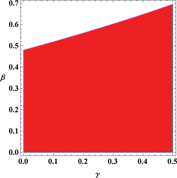
Fig. 1: Contour plot for A = 0; positron concentration  vs. nonthermal parameter
  .
.
Download figure:
Standard image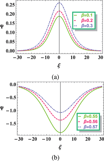
Fig. 2: Variation of  vs.
vs.
 for different values of nonthermality parameter β and for fixed values of
  ,
,  ,
,  ,
,  and
and  , (a)
, (a)  for positive potential solitary structures, (b)
  for negative potential solitary structures.
Download figure:
Standard imageIn fig. 3(a) we depict Ψ vs.
ξ for various values of positron concentration  while taking all other plasma parameters constant; the graph shows that an increase in γ decreases both the amplitude and width of positive potential solitary structures. Similarly, from fig. 3(b) it is noted that an increase in γ leads to enhancing both amplitude and width of negative potential solitary structures. To study the effect of ion thermality δ on IASWs, we plot Ψ against ξ as shown in fig. 4. It is clearly seen that higher values of δ lead to smaller amplitude positive potential IASWs as shown in fig. 4(a), while the reverse effect is observed for negative potential IASWs (see fig. 4(b)).

Fig. 3: Variation of  vs.
vs.
 for different values of positron concentration γ and for fixed values of
  ,
,  ,
,  ,
,  and
and  , (a)
, (a)  for positive potential solitary structures, (b)
  for negative potential solitary structures.
Download figure:
Standard image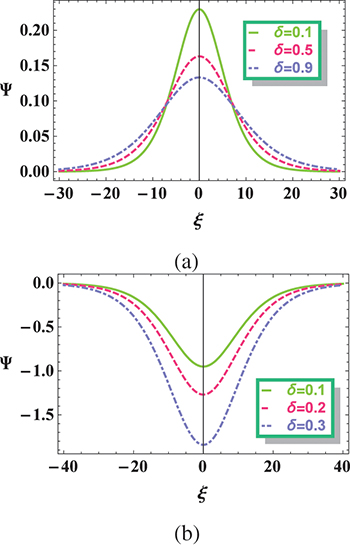
Fig. 4: Variation of  vs.
vs.
 for different values of ion thermality parameter δ and for fixed values of
  ,
,  ,
,  ,
,  and
and  , (a)
, (a)  for positive potential solitary structures, (b)
  for negative potential solitary structures.
Download figure:
Standard imageFigure 5 depicts the variation of mKdV solution  vs.
ξ for different values of β keeping all other parameters fixed. Increasing β leads to reducing the amplitude and also the width of the IASW structures.
vs.
ξ for different values of β keeping all other parameters fixed. Increasing β leads to reducing the amplitude and also the width of the IASW structures.
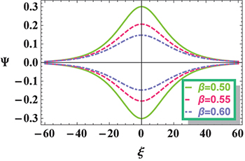
Fig. 5: Variation of mKdV solution  given by eq. (32) vs.
ξ for different values of β and for fixed values of
given by eq. (32) vs.
ξ for different values of β and for fixed values of  ,
,  ,
,  ,
,  ,
,  and
and  .
.
Download figure:
Standard imageIn fig. 6, the variation of IASW profile  of the mKdV equation (defined by eq. (32)) vs.
ξ is presented for different values of δ and fixed values of other parameters. It is clearly seen that the amplitude of both compressive and rarefactive IASWs increases with higher δ.
of the mKdV equation (defined by eq. (32)) vs.
ξ is presented for different values of δ and fixed values of other parameters. It is clearly seen that the amplitude of both compressive and rarefactive IASWs increases with higher δ.

Fig. 6: Variation of mKdV solution  given by eq. (32) vs.
ξ for different values of
given by eq. (32) vs.
ξ for different values of  and for fixed values of
  ,
,  ,
,  ,
,  ,
,  and
and  .
.
Download figure:
Standard imageFinally, fig. 7 shows how the mKdV IA solitary structure changes with magnetic field strength Ω. It is shown that the width of IASW decreases with increase in Ω while the amplitude remains unchanged with the variation of Ω. This is because A is independent of the magnetic field, therefore the amplitude has no effect on Ω. The effect of Ω on IASWs is consistent with that of ref. [36].
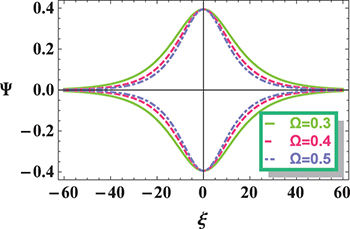
Fig. 7: Variation of mKdV solution  given by eq. (32) vs.
ξ for different values of
given by eq. (32) vs.
ξ for different values of  and for fixed values of
  ,
,  ,
,  ,
,  ,
,  and
and  .
.
Download figure:
Standard imageConclusions
In the present studies, the nonlinear IASWs are investigated in a magnetized EPI plasma consisting of warm ions, with Cairns distributed electrons and positrons. Using RPT, KdV and mKdV equations have been derived and their SW solutions are obtained. On the basis of nonthermality parameter β and positron concentration γ both polarities of solitons are observed. We study the effect of electron nonthermality parameter β, positron concentration γ, ion thermality δ and magnetic field strength Ω on nonlinear IASWs. The main results are summarized as follows:
- The amplitude of positive (negative) potential IASWs increases (decreases) as β increases.
- The amplitude of positive (negative) potential IASWs decreases (increases) as γ and δ increased.
- The amplitude of mKdV solitons increases as δ is increased, while the reverse effect is observed with increasing β.
- The amplitude of mKdV solitons is unchanged with increasing Ω, while its width is reduced.
Our results clarify the nonlinear periodic electrostatic structures that propagate in space and astrophysical environments, where magnetized EPI plasma with nonthermal electrons and positrons may exist, like ionosphere, magnetosphere and protoneutron stars [19,20,37,38].
Data availability statement: The data generated and/or analysed during the current study are not publicly available for legal/ethical reasons but are available from the corresponding author on reasonable request.