

Abstract
Natural time analysis has been recently applied for the elaboration of data recorded by means of the Acoustic Emission (AE) sensing technique while specimens and structures are mechanically loaded at levels approaching those causing macroscopic fracture. In terms of the variance  , the entropy in natural time S, as well as the entropy in natural time under time reversal
  , a complex behavior was observed, which could be understood by the Burridge-Knopoff train model and the Olami-Feder-Christensen earthquake model. Here, the AE data recorded when notched fiber-reinforced concrete specimens were subjected to three-point bending until fracture, are analysed in natural time. The analysis leads to
  , S, and
  values that are compatible with those obtained by a centrally fed Bak-Tang-Wiesenfeld sandpile model, which was theoretically studied in natural time almost a decade ago.
Export citation and abstract BibTeX RIS

Published by the EPLA under the terms of the Creative Commons Attribution 4.0 International License (CC-BY). Further distribution of this work must maintain attribution to the author(s) and the published article's title, journal citation, and DOI.
Introduction
In order to enlighten the fracture mechanisms and the crack development processes which occur in mechanically loaded specimens or full-scaled structures under severe mechanical load that eventually leads to catastrophic failures, many non-destructive monitoring techniques have been employed. The most mature among them is the Acoustic Emissions (AE) technique, which is based on the detection of the transient elastic waves produced due to the formation and propagation of cracks [1]. These waves travel within the volume of the material towards its surface in a spherical manner [2,3], where they are detected by properly attached piezoelectric sensors. The AE technique has been employed successfully both at laboratory scale [4,5] and, also, in situ for the estimation of the remaining service life and the remaining load-carrying capacity of full-scaled structures [6–10]. Thus, several AE-related parameters which can be retrieved directly from the AE recording systems, such as the cumulative energy, the cumulative number of counts and the amplitudes of the AE data, have been used for the study of the internal crack evolution processes dictating the response of the material prior to fracture [11,12]. In addition, more complex AE statistics derived from the aforementioned AE parameters are often employed, including the b-value analysis (which expresses the distribution of the recorded AE amplitudes in terms of the Gutenberg and Richter law [13–15]) and the F-function [16,17] (that represents the average frequency of occurrence of AE data in a sliding time window of a fixed number of consecutive AE data). In this letter, we focus on the application of the AE technique in conjunction with the natural time analysis [18–22]. Signal analysis in the natural time domain allows for the optimal information extraction, while at the same time it reduces ambiguity through the enhancement of the signals' spatiotemporal characteristics [22]. Natural time has been used successfully in a variety of fields, see, e.g., [22–38], including AE [39–43] ranging from remote sensing and heart dynamics [44] to the prediction of strong avalanches in cellular automata and earthquakes [45,46].
Analysing AE signals recorded from specimens made of brittle materials (e.g., rocks and rock-like materials) in natural time allows the researchers to consider the specimens under intense mechanical load as dynamical systems initially at an equilibrium state which gradually degenerates into a non-equilibrium one, as the applied mechanical load increases. In this context, impending fracture can be considered as a phase change. For this reason, the natural time of AE has been previously studied in a variety of fracture experiments for various materials like Etna basalt [39], plunged granular bed [40], marble [41,47], steel [42], cement mortar [48–50], rods of Luserna stone [43] as well as structures of technological interest [51]. Within this context and by comparing with the natural time analysis of earthquake models, we have examined in earlier works [48–50] the possibility of determining the criticality in specimens made of cement mortar and Dionysos marble under severe mechanical load until their fracture. Results showed [48–50] that the variance  of natural time may be of practical importance for identifying the entrance of mechanically loaded specimens in the stage of impending fracture, by exhibiting a behavior which could be understood either by the Burridge-Knopoff train model [52] or the Olami-Feder-Christensen earthquake model [53] when analysed in natural time.
In this study, AE signals recorded while notched fiber-reinforced concrete beams were subjected to three-point bending until fracture are analysed in natural time. In the following section, the background of natural time analysis is shortly outlined together with the results obtained for a stochastic sandpile model (note that recently there has been significant progress in understanding noise-excited systems [54] as well as appropriately describing their behavior [55,56]). Details on the laboratory measurements will be given in a later section, while the presentation of the experimental results and their discussion follows. Finally, the conclusions are summarized in the last section of this letter.
Natural time analysis: background
Consider a time series composed of N acoustic events [48]. The natural time of the k-th event of AE energy Ak
is defined by  [18,19,21,22]. Attention is focused on the pair
  where
where  represents the normalized AE energy. The variance
  of the natural time χ weighted for pk
is given as
of the natural time χ weighted for pk
is given as

In the context of seismicity,  has been suggested [57] as an order parameter where the new phase is a strong earthquake while the control parameter is the time elapsed since the stress in the focal area started increasing gradually before the strong earthquake, see, e.g., figs. 1 and 2 of ref. [57], (see, also, ref. [58] for works on
  fluctuations). In general, the scaled Probability Density Function (PDF) of
  displays [24,49,50,57] a behavior similar to the order parameter of many equilibrium and non-equilibrium systems [59–67]. Also, it has been established that when
  approaches the value 0.070, the dynamical system is reaching a critical point [68].
The entropy S in natural time is defined as [20,22,31]

where the brackets express the mean value corresponding to the distribution pk
, i.e.,  . Such a definition of entropy establishes dependency on the consecutive order of the event time series. It is, also, positive semi-definite, concave, and satisfies Lesche experimental stability [69,70]. In addition, S is causal since it is not invariant under time reversal and, therefore, the entropy under time reversal
  can be also established. This way, the entropy change under time reversal
  can unravel interesting behaviors when the system approaches a dynamic phase transition. When Qk
are independent and identically distributed random variables, both S and
can unravel interesting behaviors when the system approaches a dynamic phase transition. When Qk
are independent and identically distributed random variables, both S and  approach [71] the value
  obtained for
  and
and  , which within the context of natural time analysis is termed "uniform" distribution [20,22,31] (cf. in this case
  ).
).
The Bak, Tang, and Wiesenfeld (BTW) model [72] considers a D-dimensional lattice with a linear size L. The system starts its dynamics when a sand grain is added in the i-th block, i.e., when  ; the integer variable
  denotes the number of sand particles in the i-th block site. The i-th block will topple when it reaches instability. This condition holds when zi
equals the threshold value equal to 2D; then, zi
is decreased by 2D and its nearest neighbors (nn) increase their value by one:
denotes the number of sand particles in the i-th block site. The i-th block will topple when it reaches instability. This condition holds when zi
equals the threshold value equal to 2D; then, zi
is decreased by 2D and its nearest neighbors (nn) increase their value by one:
An avalanche will take place if one of the perturbed neighbors also gets unstable and it will end when all blocks reach stability again. The overall number of topplings represents the size s of the avalanche or synthetic earthquake. The BTW model displays a power law behavior when the system reaches the self-organized critical (SOC) state, following the key hypothesis of BTW [72],

where τ is the size exponent.
Following ref. [68], the natural time analysis of the BTW model in one- and two-dimensional lattices is here pursued, assuming the size s of the consecutive avalanches as Ak
. In the numerical simulations that were performed, a deterministic version of the BTW sandpile model is studied, in which the central block of the lattice is always seed and the first state of the lattice is filled with zeros,  . For the case D = 2, Wiesenfeld et al. [73] proved that this system exhibits a SOC state. A stochastic version of the BTW model for D = 1 is, also, studied. In this stochastic version, the conditions mentioned for the deterministic case are maintained but a new condition is also established: When a site topples, a probability p is assigned for each of the neighbors of the toppling site that the hopping grain of sand may disappear. If a uniformly distributed random number
  exceeds this threshold probability value (u > p), then the corresponding neighbor receives a grain of sand, otherwise (u < p) the grain of sand is lost and no block receives it. In other words, when D = 1 there is a probability p for a grain to disappear from the 1D chain.
Figures 1, 2, and 3 display the results of the simulations carried out for a set of one-dimensional (1D) lattices with 2000 events and a lattice of one million blocks,  . Figure 1 corresponds to the variation of
  , fig. 2 to the entropy S, and fig. 3 to the entropy under time reversal
  vs. the number N of the consecutive avalanches considered for their calculation. In all figures, both the deterministic
  and the stochastic model results for
  are presented (cf. the stochastic model results may have a number of avalanches somewhat smaller than 2000 because the total number of seeds inserted in the central block was kept constant in the simulations). The deterministic case results for the two-dimensional lattice —labeled 2D and depicted by yellow lines—are also included in these figures. The need to investigate such small p values arises from the premise to understand how the stochastic 1D model results may gradually approach those obtained from the two-dimensional deterministic case, e.g., see the blue and the green line in comparison with the yellow one in fig. 1. The following reference horizontal thick dash-dotted lines are additionally shown in fig. 1: The line labeled BTW1D corresponds to the value
  while the line labeled BTW2D to
  . The latter two values of
  were obtained from the expression

for D = 1 and D = 2, respectively. Equation (5) comes from a combination of eqs. (5), (6), and (13) of ref. [68] and provides the asymptotic  value of
  for the deterministic BTW model cases (as can be also verified from fig. 1).
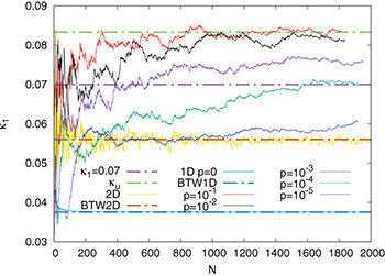
Fig. 1: The variance of natural time  vs. the number of avalanches N for the deterministic and stochastic BTW models studied. The horizontal thick dash-dotted lines labelled
  (green),
  (purple), BTW2D (brown), BTW1D (dark blue), correspond to the values 0.0833, 0.070, 0.056, 0.0375, respectively, while the yellow and the cyan lines to the results obtained from the deterministic BTW model for two (2D) and one (1D p = 0) dimensions. The
  values found when considering for
  the stochastic BTW model, discussed in the text, for
  ,
,  ,
,  ,
,  , and
, and  are shown with red, black, purple, dark green, and blue thin lines, respectively.
Download figure:
Standard image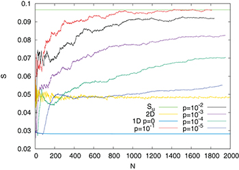
Fig. 2: Entropy S in natural time vs. the number of avalanches N for the deterministic and stochastic BTW models studied. The horizontal line labelled Su
(green) corresponds to the value 0.0966, while the yellow and the cyan lines to the results obtained for S from the deterministic BTW model for two (2D) and one (1D p = 0) dimensions. The S values found when considering for  the stochastic BTW model with
  ,
,  ,
,  ,
,  , and
, and  are drawn with red, black, purple, dark green, and blue thin lines, respectively.
Download figure:
Standard image
Fig. 3: Entropy under time reversal  vs. the number of avalanches N for the deterministic and stochastic BTW models studied. The various
  lines and curves are coloured in the same fashion as those of fig. 2.
Download figure:
Standard imageIn fig. 1, it is seen that the variation of  for the stochastic cases for N > 200 is approximately restricted in a range between 0.05 and
  ; from fig. 2, it is observed that the entropy S values stabilize in a range above 0.05 and below Su
; and from fig. 3, it is seen that the entropy under time reversal
; from fig. 2, it is observed that the entropy S values stabilize in a range above 0.05 and below Su
; and from fig. 3, it is seen that the entropy under time reversal  is approximately confined in the range above 0.08 and Su
, exceeding however the latter value in some cases. Note that in fig. 1, for the smallest p-value,
is approximately confined in the range above 0.08 and Su
, exceeding however the latter value in some cases. Note that in fig. 1, for the smallest p-value,  , the
, the  value starts from
  for small N(< 100) and then approaches
  . On the contrary, for
  after a very short initial approach to
  , the
, the  value fluctuates around
  and, finally, reaches the value
  . For
. For  and
and  , the aforementioned behavior is followed by an eventual approach to the value
  (for very large N). This behavior indicates the way the introduction of the p-value allows an interpolation between the (critical) values of
  ,
,  , and
, and  .
.
Laboratory measurements
For the needs of the present letter, concrete specimens reinforced with 7 kg/m3of long plastic fibers of length  and effective diameter
  submitted to three-point bending were studied. The specimens were beam-shaped with square cross-section and mechanically notched at their central section. The dimensions of the specimens were
  while the dimensions of the notches were approximately 25 mm in depth and 5 mm in width. The specimens were subjected to three-point bending (fig. 4) until fracture under displacement-control mode. The loading scheme was that dictated by the EN14651 standard: the initial displacement rate was equal to 0.08 mm/min, as long as the notch mouth opening displacement (NMOD) remained less than 1 mm. From this value onwards, the displacement rate was increased to 0.20 mm/min. All tests were carried out using an INSTRON (SATEC series) stiff servo-hydraulic loading frame of capacity 300 kN, while the NMOD value was recorded using an INSTRON clip-gauge.
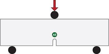
Fig. 4: Schematic diagram (not to scale) of the tested specimens showing their basic geometrical features and the location of the AE sensor considered in the present study (green circle).
Download figure:
Standard imageThe AE data studied here were obtained by an AE sensor of the R15a type attached on the immediate vicinity of the crown of the notch. Details regarding the loading protocol can be found in ref. [74].
Results and discussion
Figure 5(a) depicts the energy of the acoustic hits vs. the conventional time together with the normalized applied load  where
where  is the fracture load. In fig. 5(b), the results from the analysis of the energy of the acoustic hits in natural time, i.e., the quantities
  , S, and
  , are plotted vs. the conventional time. Finally, in fig. 5(c),
  , S, and
  , are plotted vs.
  , where N stands for the AE events considered in the calculation and
  is the total number of acoustic hits before fracture.
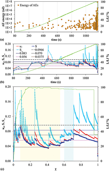
Fig. 5: Results obtained from the natural time analysis of the AE recorded during the three-point bending loading protocol. (a) The temporal evolution of the AE energies recorded (orange squares, left scale) in combination with the normalized applied load  (green line, right scale). (b) The temporal evolution of the parameters
  (red pluses), S (blue squares),
  (cyan squares) in combination with the normalized applied load
  , as in (a). See the legend for the values of the drawn horizontal lines. (c) The same as in (b) but vs. natural time. The colored areas in (c) indicate when the natural time analysis results resemble those of the one-dimensional or two-dimensional BTW model and are shown by yellow or blue shade, respectively.
Download figure:
Standard imageA detailed inspection of fig. 5(c) shows that, if a transient behavior observed before  is ignored, the quantity
  approaches
  and fluctuates around this value until
  when it departs from
  and starts to approach
  . This behavior is reminiscent of the one shown in fig. 1 for
  or
or  . Moreover, during this transition both S and
  entropies remain below Su
. From a qualitative point of view, they exhibit a variation similar to that depicted in figs. 2 and 3, respectively. Interestingly, the experimentally obtained S values (blue squares in fig. 5(c)) vary from 0.035 at
entropies remain below Su
. From a qualitative point of view, they exhibit a variation similar to that depicted in figs. 2 and 3, respectively. Interestingly, the experimentally obtained S values (blue squares in fig. 5(c)) vary from 0.035 at  to 0.06 at
  while in fig. 2 the entropy S varies from 0.03 to 0.05 or even higher for
  or
or  . After an abrupt increase at
  ,
,  , S, and
  finally reach (just before fracture) the values
  ,
,  , and
, and  which are also compatible with those obtained from the natural time analysis of the BTW model for D = 2 (see the yellow lines in figs. 1,2, and 3).
The aforementioned multitude of observations reveal that the specimen exhibits a behavior that can be qualitatively understood through the centrally fed BTW model for  and
and  dimensions whose analysis in natural time led to figs. 1,2, and 3. The fact that the BTW model for
  is initially compatible with the experimental data could be attributed to the beam shape of the specimen while the presence of the notch (see fig. 4) should be considered responsible for the central feeding since it enhances locally the stress field there. Initially, as the stress relaxes along the beam, the acoustic hits resemble those obtained from the BTW model for
  . The complex structure of the specimen allows the internal reinforcement with fibers to partially accommodate the stress field, which effectively leads to a behavior compatible with the stochastic models studied in figs. 1,2, and 3 for non-zero p values. At the last stages, after criticality has been reached, cracking is restricted over the flanks of the main macrocrack, due to shear effects along the fiber-concrete interface and the results at this stage are compatible with the BTW model for
  .
.
Conclusion
The energy of the acoustic hits detected while notched concrete specimens reinforced with long plastic fibers were subjected to three-point bending until fracture have been analyzed in terms of natural time. Interestingly, the results are compatible with a Bak-Tang-Wiesenfeld model that has been studied [68] in natural time almost a decade ago. Recapitulating, it can be said that during the initial loading stages, stresses "spread" from the notch throughout the beam-shaped specimen, activating AE sources related to either pre-existing defects or boundary slipping processes at the interface zones between the concrete and the reinforcing fibers (BTW for  ). Progressively and until the collapse of the specimen, the intensified stress field results in activation of AE sources related to the macroscopic cracks. This gradual stress concentration around the notch and the subsequently produced AEs allow for the transition from the BTW for
  to
to  .
.
Data availability statement: The data that support the findings of this study are available upon reasonable request from the authors.