

Abstract
Supersymmetric quantum mechanics (SUSYQM) provides an important method for solving the Schrödinger equation rapidly and conveniently. Based on SUSYQM, for the trigonometric Scarf potential, we find that the shape invariance with two parameters shows a new characteristic, i.e., two parameters' cross-additivity  . That is different from the parameters' change
  . The changing of the parameters with cross-additivity brings new characteristic to the wave function and energy spectrum. Based on this cross-additivity characteristic, we discuss in detail the eigenvalues and the eigenfunctions of the Hamiltonian with this potential. And then we get the two-parameter cross-additivity shape invariance again with potential algebra methods and study the energy spectrum. It is shown that the two-parameter cross-additivity shape invariance of the partner potential is completely self-consistent with its potential algebraic form. Our research indicates that the Schrödinger equation with a superpotential with two parameters shows new characteristics.
Export citation and abstract BibTeX RIS

Published by the EPLA under the terms of the Creative Commons Attribution 4.0 International License (CC-BY). Further distribution of this work must maintain attribution to the author(s) and the published article's title, journal citation, and DOI.
Introduction
The supersymmetry (SUSY) has permeated almost all fields of Physics: atomic and molecular physics, nuclear physics, statistical physics, and condensed matter physics [1–3]. During the process of solving the Schrödinger equation with supersymmetric quantum mechanical methods (SUSYQM), the most critical task is to find the superpotential of the solvable potential and to derive the shape invariance of the partner potentials based on the superpotential [4–15]. These references have shown that the solvable potentials can be solved through SUSYQM, the superpotential and shape invariant relations have been given. However, after a careful study of the shape invariance relationship of the partner potential, we find that the shape invariance of the corresponding superpotential is almost determined by the additivity of one parameter, while the values of other parameters are fixed (without additivity), such as the trigonometric Scarf potential, the hyperbolic Scarf potential, the hyperbolic Pöschl-Teller potential, the trigonometric Pöschl-Teller potential, and so on [4–15]. This is not rigorous both in the physical and mathematical sense. Since other parameters can also exhibit additivity characteristics simultaneously, they can also make the partner potentials have other forms of shape invariance. With this purpose in mind, we studied the trigonometric Scarf potential and obtained the expected results. Of course, the relevant theory of shape invariance of two parameters is certainly more complex than the shape invariance theory of one parameter. This paper will focus on the shape invariance of the superpotential with two parameters based on SUSYQM.
Another important content in SUSYQM is the potential algebra [10]. Through the potential algebra method, we can further normalize the relevant parameters in the solvable potential. Moreover, we can also use the Lie algebra theory to conduct a deeper study [11]. Similarly, at present, the SUSYQM studied by potential algebra theory is still dominated by one parameter, and there is nearly no case involving two parameters. Therefore, it is also of great necessity to study the algebra theory of the potential under two parameters in SUSYQM. In this paper, we compare the shape invariance of the partner potential and research the potential algebra of two parameters based on one-parameter potential algebra. The relevant results we obtained are also consistent with each other.
Therefore, this paper mainly involves the following aspects: In the next two sections, introductions to SUSYQM and two-parameter potential algebra are given. In the fourth section, we take the trigonometric Scarf potential with two parameters as an example for further study. In the fifth section we find that there are four cases of shape invariance. And this includes a new additive characteristic called two-parameter cross-additivity shape invariance. In the sixth and seventh sections, based on this cross-additivity, we discuss in detail the eigenvalues and the eigenfunctions of the Hamiltonian with the trigonometric Scarf potential. In the eighth section, we use the two-parameter potential algebra theory to calculate the potential and also obtain the energy spectrum and eigenfunctions. Tha last section is devoted to conclusions and discussions.
Two-parameter supersymmetric quantum mechanics
Through analysis, we find that there are many potentials with two parameters that can be solved accurately at present, such as the trigonometric (hyperbolic) Scarf potential, the hyperbolic (trigonometric) Pöschl-Teller potential, and so on. At present, almost all of the references treat them as the one-parameter cases [12]. There are only one-parameter corresponding results in the energy spectrum and the eigenwave function. In this article, we give further analyses through taking the trigonometric Scarf potential as an example which has two parameters.
Two parameters in the superpotential mean that there are two independent parameters a and b in addition to the independent variable x, that is,  . And the increasing and decreasing operators are

The partner Hamiltonians are

The partner potentials are

where the parameters a1 and b1 are two functions of the parameters a0 and b0, i.e.,  and
and  is a function of the parameters a0 and
  have the same dependence on the independent variable x. The differences between
  are the different values of the parameters a and b. There is also a corresponding relationship for
  :
:

where  is a function of the parameters a0 and b0, and
  is a function of the parameters a1, b1. We can also get
  . According to eq. (4), because there is a constant difference between the two Hamiltonian functions, their eigenvalues have also the same constant difference, and both have the same set of eigenfunctions, that is, for all values of n, there are

and

When the SUSY is not broken spontaneously, the eigenvalue of the ground-state is zero, i.e.,  . Through the iterative rule, the eigenvalue of
  is
is

The eigenfunction of  is
is

where the ground-state eigenfunction  is
is

The above is the principle of shape invariance with two parameters.
Potential algebra with two parameters
Based on the shape invariance of eq. (3), we can also adopt the relevant basis of the Lie algebra to derive the potential algebra shape invariance under the condition of the superpotential with two parameters. For this purpose, the Casimir operator J3 and the operators  are introduced. Similar to the one-parameter form [13], here we argue that these operators also contain two parameters. These operators are defined as


where sA
and sB
are constants which reflect the additive step length of parameters a and b, k is an arbitrary constant, the function χ must satisfy the compatibility equation  in which
  is a function of
  and
and  is an auxiliary variable, the operator
  is obtained from
  by introducing an auxiliary variable
  , and regarding
  independent of z and replacing the parameter
  with an operator
  ,
,

and  have the characteristics of raising and lowering operators. And J3 satisfies the following properties:

Since we consider that the parameters a and b,  and
and  , sA
and sB
are independent of each other. For example,
, sA
and sB
are independent of each other. For example,  .
.  . And for further discussion, see refs. [16,17]. The commutations of
  and J3 are satisfied with


The remaining commutation relations are equal to zero. These operators are explicitly checked,

where  is a function of
  and
and  . Suppose
  as an arbitrary eigenstate of J3, and
  play the role of raising and lowering operators, and then there are


where  and
and  are functions of eigenvalues hA
and hB
. According to
are functions of eigenvalues hA
and hB
. According to ![$\left[J_{+}, J_{-}\right] \mid\!\!h \rangle =F\left(J_{3}\right) \mid\!\!h \rangle$](https://content.cld.iop.org/journals/0295-5075/140/1/18001/revision2/epl22100481ieqn40.gif) , we obtain
, we obtain

If  , then
  and
and  . By repeating the iterative calculations, we can get

where n is a positive integer. If  and
and  is allowed to act on the state
  , the following relation can be obtained:

We can calculate the energy spectrum through eq. (23)
The above is the principle of SUSYQM under the condition of superpotential with two parameters.
The four cases of shape invariance of the trigonometric Scarf potential
The trigonometric Scarf potential is an important potential in the field of quantum mechanics and solid-state physics [18–20]. So, it is of great significance to study and discuss this potential (including its inverse potential) [21]. Studies also involve Scarf potential plus other potentials, and even extend to D-dimensional conditions [22,23]. The solution of the Schrödinger equation with the trigonometric Scarf potential through the SUSYQM method has also been discussed in many references [24–28]. The following is a brief introduction to the solution of SUSYQM of the trigonometric Scarf potential. The superpotential of the trigonometric Scarf potential is

where  . The partner potentials are

The figures of the superpotential and partner potentials are shown in fig. 1.
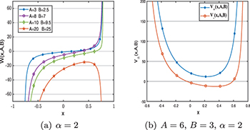
Fig. 1: The figures of the superpotential and partner potentials (a) reveal the relationship between the superpotential and A and B. (b) The figure of the partner potentials
Download figure:
Standard imageAs fig. 1(a) shows that only when B < A, W(x) can have an intersection point with the x-axis. When B > A, W(x) has no intersection point with the axis, we call the SUSY broken at this time [6], this article does not discuss such a situation.
Select  and
and  , we can obtain the shape invariance of
  , and
, and  . Furtherly, we have


However, the superpotential of the trigonometric Scarf potential contains two parameters: A and B. It is incomplete to choose only A and its consistent additivity to obtain the shape invariance and establish the energy spectrum and the eigenfunction. We define the case with only one parameter to discuss as one-parameter shape invariance.
To make a comprehensive discussion of the shape invariance of the trigonometric Scarf potential, we need to consider the case of two parameters. The specific expression for the partner potentials in eq. (25) is as follows:


To satisfy the shape invariance in eq. (3), the coefficients of the variable x in eqs. (28) and (29) have to cancel each other. So the following needs to be satisfied:

Through rigorous calculation, we can obtain four solutions that satisfy the shape invariance of eq. (3):
Case i):  .
.
Case ii):  .
.
Case iii):  .
.
Case iv):  .
.
For Case i), the solution does not exhibit additivity properties, we do not discuss it here. In Case ii), only A changes additively, while the other parameter B remains unchanged, so the situation is essentially a single-parameter additive shape invariance. This is not what this paper will focus on, as this single-parameter additive shape invariance has been discussed in too many articles before. The discussion of it can be found in ref. [12]. In Case iii) and Case iv), both parameters A and B are changing. However, parameter A is increasing in Case iii), while parameter B is decreasing, that is, the additivity is more complex. We will study this case in our later research.
In Case iv), the parameters A and B not only exhibit additive changes, but also show staggered characteristics. Therefore, the study of this situation will be more complicated than the existing two-parameter pure additive change situation. This computationally rigorously derived a new shape invariance form of the trigonometric Scarf potential, which has never been discovered by supersymmetry researchers before. Therefore, our research team calls it as two-parameter cross-additivity shape invariance. Let us now turn to what exciting and different results this new shape invariance form can bring us from the previous one-parameter additive shape invariance.
Two-parameter cross-additivity shape invariance of the trigonometric Scarf potential
According to the shape invariance requirements of eq. (3), and the additivity characteristic of the parameters  and
and  . Although we say that they show pure additivity characteristics, it is not only simply additivity, but also crossover additivity. The increase of the latter A is always based on the former B. Similarly, the increasing of the latter B is always based on the former A. Using the iteration, we can derive recursive relations between the parameters that satisfy the shape invariant requirement which are shown in table 1.
Table 1:. The parameters expressions of the partner potentials 

| expressions |

|

|

|

|

|

|
| ... | ... |

|

|

|

|
From table 1, we find  . As can be seen from the relationships listed above, we need to discuss the index partition parity.
1) When n is an even number, we set  ,
,


2) When n is an odd number, we set  ,
,

The partner potentials are shown in fig. 2.
Note that the abscissa represents x.
As can be seen in fig. 2,

this means that  , which is not allowed.While
  is greater than 0, the correct energy level can be obtained. The partner potentials shown in fig. 2 inspire us to also discuss the parity of the energy level
  .
.
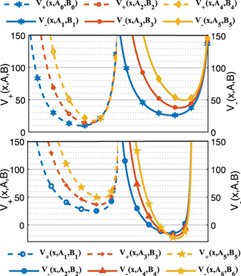
Fig. 2: The partner potentials for  .
.
Download figure:
Standard imageThe eigenvalues of the two-parameter cross-additivity shape invariance
From eq. (7), we have

Further, we can obtain

By analogy, we can conclude that when k is an even number

when k is an odd number,

The energy levels are shown in fig. 3.

Fig. 3: A part of energy levels for  . Note: dotted lines indicate non-existent energy levels, and solid lines indicate possible energy levels.
Download figure:
Standard imageBased on fig. 3 and eqs. (37)–(39), our discussion can be divided into the following four cases.
i) When k is an even number and n is an even number, too,  .
.
ii) When k is an even number, n is an odd number and small enough, that is, to ensure that  . The wave function does not exist, namely, the wave function diverges. It is worth noting that, as can be seen from fig. 3, when k is an odd number, as k increases, the situation
  will definitely occur, which means
  . The minimum value of n that can satisfy the above situation is
 ![$n=\left[A_{0}-B_{0}\right]$](https://content.cld.iop.org/journals/0295-5075/140/1/18001/revision2/epl22100481ieqn82.gif) .
.
iii) When k is an odd number and n is an even number,  .
.
iv) When k is an odd number and n is an odd number, too,  . The summary of the energy levels are shown in table 2.
Table 2:. A summary of the energy levels. Note  .
.
| Exisiting | Non-exisiting |
|---|---|
| energy levels | energy levels |

| None |

|

|

|
![$\left(n<\left[A_{0}-B_{0}\right]\right)$](https://content.cld.iop.org/journals/0295-5075/140/1/18001/revision2/epl22100481ieqn90.gif)
|
![$\left(n \geq\left[A_{0}-B_{0}\right]\right)$](https://content.cld.iop.org/journals/0295-5075/140/1/18001/revision2/epl22100481ieqn91.gif)
|
The eigenfunctions of the trigonometric Scarf potential based on the two-parameter cross-additivity shape invariance
For  , whether the eigenwave function exists will be further discussed below. And we also can deduce the ground-state wave functions

where  is the normalized constant. Because we have given A > B in advance, i.e., A0 > B0, when
  , the zero-energy ground-state wave functions
  are normalizable. But, when
  , the zero-energy ground-state wave functions
  are unnormalizable. Based on eq. (8), the excited states of the trigonometric scarf potential can be obtained by using the rising operator
  . We will discuss this in detail.
According to table 1, the alternating additivity of the coefficients of the partner potentials can be summarized as

There are two classes of the ground-state wave functions  .
.
When  , if A0 > B0, i.e., An
> Bn
, the ground-state wave functions
, if A0 > B0, i.e., An
> Bn
, the ground-state wave functions  are normalizable. The first five zero-energy ground-state wave functions are shown in fig. 4(a).
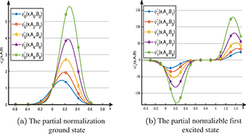
Fig. 4: The partial ground-state wave functions and the first excited state wave functions.
Download figure:
Standard imageWhen  , if A0 > B0, i.e., An
< Bn
, the ground-state wave functions
, if A0 > B0, i.e., An
< Bn
, the ground-state wave functions  are unnormalizable.
The first excited state wave functions can be written as

There are two classes of the first excited state wave functions  .
.
Although the zero-energy ground-state wave functions  (where
  is normalized when An
> Bn
is satisfied,
is normalized when An
> Bn
is satisfied,  is not normalized. The reason is that
  acts on
  , and
, and  and
and  in
in  satisfy
  ,
, is spontaneously broken.
Conversely, although the zero-energy ground-state wave functions  (where
  is not normalized when An
< Bn
is satisfied,
is not normalized when An
< Bn
is satisfied,  is normalized. The reason is that
  acts on
  , and
, and  and
and  in
in  satisfy
  . The first five normalizable wave functions in the first excited state are shown in fig. 4(b).
What about the second excited state? Whether its characteristics are similar to the ground state or the first excited state, let us explore further. The second excited state wave functions are

There are two classes of the second excited state wave functions  .
.
i) When An
< Bn
is satisfied, the first excited state wave functions  (where
  are unnormalizable, functions
  are normalizable.
ii) Conversely, although the first excited state wave functions  (where
  is normalizable when An
> Bn
is satisfied,
is normalizable when An
> Bn
is satisfied,  is unnormalizable.
At this point, this indicates that the cross-additive change of two parameters will lead to a part of the wave function breaking, and which part of the wave function breaking should also be discussed in terms of odd and even energy levels. The m-th excited state wave functions

There are two classes, too.
i) When m is an even number, if the parameters satisfy An
< Bn
, although the  excited state wave functions
  , where
  are unnormalizable
  are normalizable.
ii) When m is an odd number, if the parameters satisfy An
< Bn
, although the  excited state wave functions
  (where
  are normalizable,
  are unnormalizable. A summary of the ground-state and the excited state is shown in table 3.
Table 3:. A summary of the ground-state and the excited state. Note .
.
| Normalizable | Non-mmormalizable |
|---|---|
| state | state |

|

|
|
|
The potential algebra of the trigonometric Scarf potential with two parameters
For  , we can define operators
  and
and  is a Casimir operator):


Since  embodies the additive characteristic of parameter interchanging, operators must also reflect the additive characteristic of such interchanging, i.e.,
  and
and  . Therefore, for the calculation of the first excited state energy spectrum with the potential algebra method, we need to interchange the coefficients in
  to reflect additivity, while we need not interchange the coefficients in
  . According to eqs. (45) and (46), we have

We can obtain  . Further, we have

When calculating the energy spectrum of the second excited state with the potential algebra method, the coefficients in  need to interchange again based on the first excited state to reflect the corresponding additivity characteristics. However, the coefficients in
  remain the same as those in the first excited state and need not interchange to correspond to each other, so we still have

From eq. (23), we know

If we want to determine the energy spectrum, it is obvious that we also need to consider the characteristics of cross-correspondence between two coefficients. Therefore, we have


Set

and we get
This result is the same as eqs. (37)–(39). This shows that the shape invariance of the partner potential derived in this paper is consistent with the shape invariance of the potential algebra, and the theory is self-consistent.
Conclusions and discussions
The shape invariant potential obtained by changing the two parameters at the same time brings new physical features to the wave function and energy spectrum, which is by no means a repeated study of the original super potential. In this paper, we take the Scarf potential as an example, deriving the shape invariance of the partner potentials of the two-parameter superpotential. The problems related to shape invariance are deeply studied. Our results exceed the theoretical expectation of two-parameter shape invariance: the parameters show cross-additive characteristics. For the shape invariance of the partner potentials of the trigonometric Scarf potential, we focus on the shape invariance with two parameters, and derive the energy eigenvalues and the eigenwave functions. It is worth noting that in the shape invariance of partner potentials, the two-parameter's additivity is alternating. These additive characteristics also bring new features to the eigenwave functions. These have been discussed in detail in the paper. Further, we study the potential algebraic shape invariance of the partner potentials of the trigonometric Scarf potential, which also focuses on the algebraic shape invariance of the potential with two parameters, and derive the same energy eigenvalues as for the partner potentials. The analysis of the example also shows that many of the solvable two-parameter superpotentials involved may not be comprehensive enough, and the shape invariance of the solvable potential in many references [4,12,16,17] needs further investigation. It also shows that the Schrödinger equation with two-parameter superpotential requires further investigation. According to the recent results of our study group, a further study of the shape invariances of the two parameters is well expected.
Data availiability statement: All data that support the findings of this study are included within the article (and any supplementary files).