

Abstract
We propose a computational quantum field theoretical approach to obtain a microscopic insight into the creation process of electrons and positrons as well as their subsequent motion inside a supercritical external field with space-time resolution. A machine-learning–based method permits us to address fundamental questions such as where inside the interaction region the particles are being created and what their initial velocity distribution is. It suggests that the particles' most likely birth positions change in time during the dynamics. At early times the particles' birth density is roughly proportional to the square of the force field, but in the long-time and steady state production regime their possible birth locations narrow down significantly. Counterintuitively, this leads for longer times to the occurrence of "birth-free" zones within the field, where particles are no longer created even though the electric field is maximal there. The genetic-programming–based symbolic regression algorithms first learn multiple sequences of partially dressed positronic spatial probability densities as training data and then exploit their features as a function of the dressing strength in order to predict the particles' true distribution in space and momentum.
Export citation and abstract BibTeX RIS
For a long time, it was assumed that it is not easy to obtain any unambiguous space-time resolved information about the very creation process of elementary particles inside supercritical electromagnetic fields. The interaction zone had to be viewed as a black box environment and any dynamical information about the generated particles was accessible to theoretical study only once the particles had escaped this zone. Outside the interaction zone the particles no longer interact with the field, such that asymptotic approaches (S-matrix) can provide us with some information about the particles' spatial, spin, or energetic features. This severely restricted access stems from the well-known problem that inside the highly interacting pair creation region, where the number of particles changes, it has not been possible to date to uniquely distinguish between electrons and positrons. While the total current and charge density for the combined system of all particles can be defined in an unambiguous manner, the required definition of more useful probability densities for each particle species separately has been non-trivial. Due to the absence of any appropriate theoretical framework, fundamental questions about the particles' most likely location and velocity at birth inside the interaction zone have not been directly accessible for study.
In this letter, we propose a machine-learning–based scheme that might have the potential to overcome this conceptual bottleneck. We illustrate this proposal for a simple model system of the electron-positron pair creation process and obtain some first microscopic insight into the birth process of the particles as well as their subsequent acceleration dynamics after their creation. This break-down process of the QED vacuum in strong external fields is also of recent experimental interest [1,2] due to the exciting progress in the development of new high power laser systems with ever growing intensities [3].
After a discussion of our methodology, we present the predicted physical implications and review the three components of the technical aspects of this approach (computational quantum field theory, quasi-densities and symbolic regression-based machine learning). Finally, with the hope of motivating further theoretical studies, we discuss new challenges that can now be addressed using this theoretical tool.
The quantum field theoretical operator  as a function of time t and the one-dimensional spatial coordinate z may be expanded and computed [2] as


 and
and  are the complete set of wave functions evolved in time under the full Hamiltonian
  , where the last term is the interaction energy and e and m are the positron's charge and mass. The abruptly turned-on electrostatic potential V0
V(z) (with
, where the last term is the interaction energy and e and m are the positron's charge and mass. The abruptly turned-on electrostatic potential V0
V(z) (with  and
and  ) is related to the spatial profile of the corresponding spatially localized supercritical electric field as
  . The maximum amplitude of this electric field is given by
  , where 2d is the spatial extension of the field. It is related to the chosen asymptotic value to the potential as
  , which makes this field supercritical. The initial states
  and
and  are the energy eigenstates of the force-free Dirac Hamiltonian, given by
  , where p labels their momentum. They fulfill
  and
and  with
with  .
.To generate the training sets for machine learning approach in the following discussion, we define the following quasi-density  for the positrons and
  for the electrons. They rely on the following partially coupled Hamiltonian
  , which differs from the full Hamiltonian only by the (variable) strength of the electric field, given by α,

This configuration is supercritical only if the dressing field strength satisfies  . Obviously, for
  this Hamiltonian
  becomes identical to the fully dressed Hamiltonian H used to determine
  . If
. If  , the potential is subcritical and the energy of the eigenstates of
  can be used to separate unambiguously between purely positronic and electronic states. These partially dressed eigenstates are defined as
  and
and  , with
  and
and  .
.
We next define the positronic/electronic portions of the field operator for each parameter  by projecting the total field operator
  onto the manifold of the set of these partially dressed states, i.e.,


 and
and  can then be defined via the expectation values with respect to the initial state
  , which is equal to the vacuum state,

With these quasi-densities (carrying the units of 1/length), a machine learning technique (outlined below) is used to construct the predicted positron and electron densities  and
and  at any moment of time after the field is switched on inside the interaction zone. An example of such a computation is displayed in fig. 1. On the top of fig. 1(a), we also included the spatial profile of the chosen two-peaked electrostatic field
  for
for  that was responsible for the particles' creation as well as their after-acceleration. The characteristic spatial and temporal scales for the dynamics are naturally provided by the fermions' Compton wave length
  and the corresponding time
  . This field has a spatial extension of
  and an amplitude of
  pointing in the negative z-direction. As the maximum energy (5mc2), which a positron can absorb from the force field, exceeds 2mc2, this field is supercritical and therefore acts as a permanent particle source, which constantly emits the created positrons to the left and the created electrons to the right.
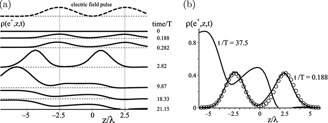
Fig. 1: (a) Seven snapshots of the positrons' spatial number density  inside and outside of a supercritical and spatially localized electric field. The two-peaked electric field pulse
  for
for  and
and  for
for  is shown above, where
  and
and  . (b) The long-time steady state density
  (for
(for  ) and the birth density
  (for
(for  ). The open circles represent the square of the electric field pulse E2(z), convoluted with the positron's point spread function
  , see ref. [4].
Download figure:
Standard imageAs one might expect, after the external field is turned on, there are three distinct temporal regimes: the sole birth process, followed by the combination of birth processes and additional after-acceleration, and finally the formation of the steady state, which can be characterized by a well-understood global pair creation rate.
During the very early time regime, where the particles do not have enough time to escape from their birth locations, the similar shapes of the positrons' spatial number density  suggest that the positrons grow in a rather shape-invariant manner, i.e.,
  . The two-peaked structure of the birth density
  suggests that it is the (square of the) electric field strength at each position that characterizes the spatial dependence of the local birth rate. The good match of the data in fig. 1(b) with the open circles shows that
  is indeed quasi-proportional to E2(z). We also found that the respective birth densities for each particle species are identical, i.e.,
  .
.
In the second temporal regime, the positrons have sufficient time to move and to be accelerated by the electric field toward negative z. Due to symmetry considerations associated with the spatial profile of our electric field, we would expect the symmetry  between the electrons and positrons, which is confirmed by our numerical data. The ratio of the distance traveled by the front of this distribution divided by the corresponding time interval suggests that the positrons evolve with a velocity close to the speed of light c.
The third (long-time) regime is characterized by the final formation of the steady state  . Except for the region ahead of the wave front, for
  , the final density
  becomes constant
  in space, which is expected as the positrons travel force-free there. As inside the electric field
  describes particles that continue to be created at a constant rate as well as particles that have traveled, a unique characterization of their birth regions is difficult. In fact, while one could have guessed the shape of
  , the resulting steady state distribution
  is truly unexpected and counter-intuitive.
There are two quite remarkable features of  . First, as we show in fig. 1(b), at those regions (around
  ) where the electric field is largest,
  actually has local minima. Furthermore, around
  , where the electric field completely vanishes, we observe a local maximum in the positronic density. This counterintuitive observation has important implications. It suggests that it is non-trivial to use a global Schwinger-like rate to approximate a local (E0-dependent) rate in powerful state-of-the-art QED and plasma codes [5–8].
Second, we observe that as the created particles vacate the interaction zone, a fully depleted region  is developed where the density basically vanishes, suggesting that the positrons can no longer be created in this particular region inside the electric field. This shows that while this region served as the major birth zone during earlier times, the particles ceased to be born in this "birth-free" zone, even though the electric field's amplitude is there still of maximum supercritical strength E0.
The observed occurrence of this (birth-free) zone is also suggested by energetic considerations. The energy distribution of the created positrons can be characterized by that portion of the negative energy manifold, which is up-lifted by the (positive) potential energy  associated with our electric field with
  . If eV0
V(z) > 2mc2 this portion can become degenerate with some of the lowest positive energy states, which begin at mc2. This means that it can lift the upper edge of the negative continuum up to a value
. If eV0
V(z) > 2mc2 this portion can become degenerate with some of the lowest positive energy states, which begin at mc2. This means that it can lift the upper edge of the negative continuum up to a value  and therefore opens the (degenerate) Klein-tunneling regime for the positrons, created in the range
  . As the largest permitted energy of the created positrons is
  , they cannot be created at locations larger than
  , for which
  . This point
  matches nearly perfectly the beginning of the birth-free region in fig. 1(b).
Next we will examine the same three stages of the time-evolution from the perspective of the positrons' momentum distribution  . It can be computed from the field operator
  in its momentum presentation, defined similarly to
  in eq. (1a), but based on the states
  and
and  . The associated total number of positrons,
  should be obtained consistently from either density. This agreement of both integrals is not obvious as
  and
and  were obtained by machine learning techniques. Therefore, the validity of this equality can be viewed as a criterion of the accuracy of these techniques themselves. Quite remarkably, at early times the birth distribution is not symmetric around
  , as presented in fig. 2. This means that the particles' most likely velocity at birth is actually not zero, but their preferred birth momentum (
 denoted by the arrow in the figure) follows the direction of the external field (and therefore the electric force), leading to an interesting asymmetry
  . We do not have any intuitive understanding for the mechanisms favoring this particular momentum.

Fig. 2: Three temporal snapshots of the positrons' momentum density  for the same electric field configuration as in fig. 1. For comparison, the open circles are the predictions according to Hund's asymptotic theory [9] given by
  , where
  is the quantum mechanical transmission coefficient [10] associated with an incoming electron scattering off the two-peaked E(z).
Download figure:
Standard imageWe should note that, in contrast to the electric-field dependent  , the momentum birth density
  seems to be rather independent of the particular shape of the electric field. We have compared this momentum distribution with that of positrons that were created by a different field configuration, where the electric field was not two-peaked but constant for
  and found a remarkably similar shape.
As in the second stage the positrons are accelerated to the left, their momentum distribution deforms and shifts to the negative momenta until the final shape of the steady state  is reached asymptotically. We note that
  matches the predictions of other traditional approaches, such as the S-matrix or the transmission-coefficient–based Hund's rule [9,10], shown by the open circles in fig. 2.
Let us now return to a brief summary of the technical aspects of this approach. There are three components to it: computational quantum field theory, quasi-dressed densities and machine learning. Computational quantum field theory is a well-established space-time lattice-like technique based on numerical solutions to the Dirac equation to calculate the electron-positron field operator  . This method was developed about two decades ago and has been used routinely in studies of heavy ion collisions and pair creation studies of numerous field configurations [11,12].
The second component is the definition and the calculation of quasi-dressed densities  for the positrons. Using a projection of the (fully dressed) electron-positron field operator
  onto the Hilbert space of partly dressed energy eigenstates
  of positive energy (see eqs. (2) above), one can introduce unambiguously a positronic part of the operator,
  . As each value of
  characterizes its own set of energies (labeled by
  ), the operator
  does depend on
  . These positronic (partly-dressed) states
  can be calculated as the energy eigenstates for the fully coupled Dirac Hamiltonian, but the amplitude of the electric field (denoted by
  ) is subcritical, instead of the supercritical value E0 used to compute
  . This limits the available amplitudes
  and therefore
  to those values
  for which the potential energy satisfies the condition for sub-criticality. Ideally, if the dressing parameter
  were to match the true amplitude of the dynamical field E0, then the resulting expectation value
  for
for  would describe the true positron density
  . On the other hand, due to the energy degeneracy between the lower and upper Dirac continuum states, a direct calculation of the eigenstates
  for supercritical values of
  is unfortunately not possible yet. As the dressing parameter
  has to be less than the true amplitude E0, therefore
  is just a "quasi-dressed" density. Nevertheless, for a given value of
  ,
,  has an unambiguous and important interpretation; it becomes the true physical density at time t, if the amplitude of the supercritical electric field E0 is reduced instantly to the new value
  . The (well-known) limit of
  (based on the projection onto force-free states
  and its interpretation as particle density after the field is turned entirely off suddenly to zero) was already discussed in prior studies [11]. We should note that these densities can be qualitatively quite different compared to the true densities discussed above as we show in fig. 3. In fact,
  reveals a much more intuitive behavior than the (force-free–based)
  . The key challenge is to use the computable data
  (or equivalently
  ) for a wide range of dressing parameters
  and to predict the desired density for
  , for which the projection operator
  cannot be directly constructed due to the energy degeneracy of both Dirac continua mentioned above.

Fig. 3: (a) The momentum pseudo-densities  (at time
  ) for eleven (equidistant) dressing strengths
  , which serve as the training set for the genetic programming. The thicker graph is the prediction for the real physical density, associated with
  . For comparison, the open circles are the steady state distribution based on the long-time asymptotic Hund theory [9,10]. The rectangular electric field was constant,
  between
  and d, with
  .
.
Download figure:
Standard imageThis brings us to the third component of this theoretical approach, the machine learning algorithms. These algorithms obtain, as training sets, the (under-dressed) quasi-densities for the limited range of  . The goal for them is to learn the densities' main characteristics and trends as
  is increased for each position z (or momentum p) and at each time. After the learning is completed, they can be used to predict the true spatial or momentum density for
  . We found that evolutionary-programming–based symbolic regression provided more reliable predictions than neural networks [12]. Here for each position (or momentum) and each time, the functional dependence of the quasi-density on
  was obtained and then predicted for
  .
.
In this (symbolic regression) approach [13–15], a pool of search candidates for the density was represented by parse-trees, which were then subjected to multiple sequences of cross-overs, mutations and cloning operations until the optimum expression was computed. We found that the complexity of the optimal functional form was rather sensitive to the particular space-time (or momentum-time) point.
In our fig. 3, we present the training set of eleven quasi-momentum probabilities  for time
  associated with a rectangular electric field configuration with
  . Here the requirement of subcriticality
  limits the permitted dressing parameters to
  , leading to the eleven projections. We see that the magnitude of the unphysical large contributions to
  for positive momenta decreases as the dressing parameter
  is increased. As for long times (such as
  ) most positrons have been accelerated to the left, we consider these positive momenta as rather unphysical. It is important to stress that therefore an increase of
  makes
makes  more physical. We have also included in the figure the true physical momentum density as predicted by the machine learning algorithm. We see that all relevant momenta are negative as one would expect. As a side note, we observe that the twelve densities consistently match for larger negative momenta, as the corresponding positrons are located in the force-free region
  , where the positive energy eigenstates match and the projector
  becomes independent of
  . We have increased the number of training sets to 20 and the final answer stays unchanged.
We have also included by the open circles the corresponding prediction by the analytical Hund theory. Its nearly perfect match with the predicted density further confirms the validity of the machine learning approach. Nevertheless, as we have obviously entered a completely unexplored territory inside the pair creation zone, the question about the reliability of the new machine-learning–based predictions needs to be further addressed. We have compared the predictions of algorithms, based on genetic programming and neural networks [12] and found quite similar results. In addition to the asymptotic Hund theory, we have also examined the analytically accessible well-known vacuum polarization regime and found again consistent data for the total charge density obtained by traditional methods.
While modern machine learning approaches have just begun to become new tools in some areas of physics, to the best of our knowledge, this work is the first application to a time-dependent quantum electrodynamical theoretical problem. We view the present data just as a first proof of principle that it might be possible to study the very birth process of particles not only with full temporal but also spatial resolution inside the force zone. To keep our analysis as simple as possible, we have considered only those classes of external fields that vary in the spatial direction and that are temporally homogenous after they are turned on. While the computational effort in terms of computing time (about 5–10 CPU hours on a 24 node Intel Xeon Gold 6248R cluster) is extensive, as for each space-time point entire sequences of quasi-densities need to be calculated and consecutively fed into the machine learning algorithms, there is no principal obstacle of generalizing this computational technology to study more complicated geometries of electromagnetic field configurations, where other approaches (such as Hund's theory) cannot be applied. As in these scenarios the Dirac Hamiltonian is time-dependent, the corresponding sets of dressed states have to be calculated as instantaneous eigenstates for each moment in time separately in addition to the required range of dressing parameters  . But the potential to obtain first access to the dynamics inside the laser focus should more than justify this enormous computational effort.
The introduction of novel quantities such as probability densities of electrons or positrons as a function of the position or the momentum inside a highly interacting environment will likely motivate further theoretical challenges. For example, in our opinion, it would be very worthwhile to examine if there are some underlying new fundamental equations, that can govern the time evolution of these quantities directly. It is likely that, in this search, machine learning tools might play again a central role.
We finish this work with a remark that in traditional atomic and molecular physics microscopic insights about the electronic motion inside the atoms and the laser focus have been very valuable for the development of new means to control some mechanisms and one can foresee now similar developments also for quantum field theoretical processes. The momentum distributions can also be of practical significance as a possible link to future experiments.
Acknowledgments
We would like to thank Profs. N. Christensen, Z. L. Li and Y. J. Li for many helpful discussions. CG would like to thank ILP for the nice hospitality during his visit to Illinois State University and acknowledges the China Scholarship Council program for his PhD research. This work has been supported by the US National Science Foundation and Research Corporation. Partial funding also comes from the Fund. Res. Funds for the Centr. Univ. (20226943). We also acknowledge generous access to the HPC supercomputer cluster provided by ISU.
Data availability statement: All data that support the findings of this study are included within the article (and any supplementary files).