
Abstract
The nonlinear stability of current-driven ion-acoustic waves in collisionless electron–ion plasmas is analyzed. Seminal simulations from the 1980s are revisited. Accurate numerical treatment shows that subcritical instabilities do not grow from an ensemble of waves, except very close to marginal stability and for large initial amplitudes. Further from marginal stability, one isolated phase-space structure can drive subcritical instabilities by stirring the phase-space in its wake. Phase-space turbulence, which includes many structures, is much more efficient than an ensemble of waves or an isolated hole for driving subcritically particle redistribution, turbulent heating and anomalous resistivity. Phase-space jets are observed in subcritical simulations.
Export citation and abstract BibTeX RIS
1. Introduction
Ion-acoustic turbulence is a central paradigm of plasma physics and controlled fusion. When ion and electron temperatures are similar, linear theory predicts that ion-acoustic waves are stable (except if the velocity drift between electrons and ions is at least of the order of the electron thermal velocity), due to strong ion Landau damping [1]. As a consequence, ion-acoustic turbulence does not receive much attention in the context of magnetically confined fusion plasma. However, stability is a nonlinear issue. Indeed, the growth process of structures in phase-space can circumvent linear theory [2–7], leading to nonlinear, or subcritical instability. Furthermore, ion-acoustic waves constitute the basis for dominant fluctuations in confined plasmas. Indeed, drift-waves arise from the ion-acoustic branch, modified by inhomogeneities and geometry effects. In particular, collisionless trapped-ion and trapped-electron modes are driven by wave-particle resonance, in the same way that the current-driven ion-acoustic is. Therefore, the understanding of phase-space structures and their impact on ion-acoustic turbulence is an important step toward the advance of the nonlinear kinetic theory of collisionless plasmas.
One idea concerning subcritical processes follows from the properties of phase-space structures or granulations, which are non-wave-like fluctuations. These structures can exchange momentum and energy via channels which differ from those of familiar linear wave-particle resonance, and so can tap free energy when wave excitation cannot [2]. A structure of particular interest is a BGK-type island of negative phase-space density perturbation, referred to as a hole [2, 4, 8–14] or a phase-space vortex. These coherent structures are spontaneously formed by nonlinear wave–particle resonant interactions, which trap particles in a trough. These trapped particles in turn generate a self-potential, leading to a self-sustained structure. Like a fluid vortex, a phase-space hole is not attached to a wave or a mode. The mean velocity of the hole can evolve away from the resonance, and grow by climbing up the gradient of a particle velocity distribution.
The impact of PS holes is not limited to stability. PS holes can drive anomalous transport [15, 16], drive anomalous resistivity [17], modify the saturation amplitude [18], yield amplitude oscillations or chaos [19], shift the mode frequency [11], and couple with zonal flows [20]. These impacts are relevant in the context of energetic particle-driven activities in space and magnetic fusion plasmas [21], collisionless magnetic reconnection [22], collisionless shock waves [23], alpha-channeling [24] and drift-waves [25].
Multiple structures can coexist and interact, leading to rich nonlinear phenomena, which we refer to as phase-space turbulence. In phase-space turbulence theory [26], the system is treated as an ensemble of structures in phase-space, rather than an ensemble of waves, as in quasi-linear theory. We can contrast phase-space turbulence with conventional approaches in terms of the Kubo number K ∼ ωbτc, which measures the coherence of turbulence. Here, ωb is the bounce frequency of trapped particles, and τc is the correlation time of a structure. Conventional theories that rely on linear waves and their nonlinear extensions (mode coupling, weak and strong turbulence theories) require K < 1 for their validity. This condition is easily violated when wave-particle interactions are strong. Phase-space turbulence theory concerns the ubiquitous K ≳ 1 regime.
In this paper, we consider the ion-acoustic instability in one-dimensional (1D), collisionless electron–ion plasmas with a velocity drift. Ion-acoustic waves are longitudinal electrostatic waves, which are commonly observed in space and laboratory plasmas. Theory and experiments indicate that ion-acoustic waves are key agents of magnetic reconnection (via anomalous resistivity) [27], turbulent heating [28], particle acceleration [29], and play important roles in the context of laser–plasma interaction [30]. Linear instability requires that the velocity drift vd exceed some finite threshold vd,cr. However, nonlinear theory [31, 32] predicts that phase-space density holes can grow nonlinearly, even for infinitely small drifts. In such plasmas, electron and ion structures behave like macroparticles and scatter each other, leading to dynamical friction (in addition to the usual quasi-linear diffusion), which drives anomalous resistivity [17]. From a momentum point-of-view, phase-space holes grow by exchanging their momentum with other species or with the wave pseudo-momentum [33]. From an energetics point of view, growing structures continuously emit undamped waves by the Cherenkov process, leading to the growth of total wave energy [7, 17]. Holes can also be thought of as quasi-particle modes of zero or negative energy [9]. The hole growth rate was obtained far from [32] and close to [34] linear marginal stability. In the 1980s, particle simulations of the nonlinear electron-ion instability, with mass ratio mi/me = 4 and temperature ratio Ti/Te = 1, were performed [3, 10]. To the credit of the authors, these simulations were performed three decades ago, when computing power was roughly 7 orders of magnitude lower than today. These simulations agree qualitatively with the theory, and nonlinear growth was observed for vd > 0.4vd,cr, that is, far from linear marginal stability. Electron holes were reported to grow in a similar way from either a seed phase-space hole, or from random fluctuations, even with low-amplitude initial fluctuations (eφ/T ≪ 10−2).
However, our work suggests that these earlier particle simulations likely suffered from numerical issues, such as noise associated with a small number of particles, leading to spurious conclusions. In particular, nonlinear growth is found to be much more sensitive to initial conditions than suggested in [3, 10]. We observe that subcritical instabilities are absent when the initial perturbation consists of an ensemble of sine waves with random phases, except close to linear marginal stability (vd > 0.9vd,cr) and for large initial amplitudes (eφ/T ∼ 1).
In contrast, a seed local negative perturbation (hole-like) in the electron phase-space can grow nonlinearly, even far below marginal stability (vd = 0.38 vd,cr) and for small initial amplitudes (eφ/T ∼ 10−3). Depending on the initial conditions, a growing hole may keep most of the phase-space relatively intact (local hole growth), or, on the contrary, may lead to a turbulent state with significant potential energy eφ, particle redistribution, heating and anomalous resistivity (global subcritical instability). Such system-wide effects are observed for vd = 0.76vd,cr. However, the effects of the seed phase-space perturbation are indirect. A multitude of small holes emerge from the wake of the evolving seed perturbation. It is this phase-space turbulence that drives the subcritical instability. In other words, phase-space turbulence, rather than turbulence in the sense of a spectrum of incoherent waves, leads to substantial nonlinear growth (in general). In the turbulent state, we observe phase-space jets, which are elongated structures that enhance redistribution and anomalous resistivity [35].
2. Model
2.1. Model description
The model describes the collisionless evolution of a two-species, 1D electrostatic plasma. In addition to academic interest, a 1D model is relevant for plasma immersed in a strong, relatively homogeneous magnetic field [36]. The evolution of each particle distribution, fs(x, v, t), where s = i, e, is given by the Vlasov equation,

where qs and ms are the particle charge and mass, respectively. The evolution of the electric field E satisfies a current equation,

where ωp,s is the plasma frequency and n0 is the spatially averaged plasma density. The initial electric field is given by solving Poisson's equation. We denote δfs ≡ fs − f0,s and
 , where
 is the initial velocity distribution, and
 is the spatial average of fs. In a 1D periodic system, a spatially uniform current drives a uniform electric field, which oscillates at a frequency ωu = ωp,e(1 + me/mi)1/2. This rapid oscillation of both the uniform electric field and the uniform current is of little interest here [37]. Numerically, the average part of E is set to zero, following common practice [10, 38, 39].
2.2. Numerical simulations
On the one hand, in [6, 40], we described, verified, validated and benchmarked a semi-Lagrangian kinetic code COBBLES, capable of long-time simulations of 1D plasmas. A particular feature of this code is that the surface elements of phase-space density are locally conserved, up to the machine precision. Hereafter, we refer to these simulations as Vlasov simulations. On the other hand, to reproduce the results of [3, 10], we developed a simple particle-in-cell code, PICKLES (Particle-In-Cell Kinetic Lazy Electrostatic Solver), which can be switched between full-f and δf treatments. Hereafter, we refer to these simulations as full-f PIC simulations and δf PIC simulations, respectively. We denote the number of marker-particles per species as Np. The PIC code is used only in section 3.2. The rest of this paper is based on Vlasov simulations.
Hereafter, we adopt the physical parameters of [3, 10]. The mass ratio is mi/me = 4 (small mass ratio improves numerical tractability and the readability of phase-space contour plots). The system size is L = 2π/k1, where
 . The initial velocity distribution for each species is a Gaussian,
![$f_{0,s}(v)=n_0/[(2\pi)^{1/2}v_{T,s}]\exp [-(v-v_{0,s})^2/2 v_{T,s}^2]$](https://content.cld.iop.org/journals/0741-3335/56/7/075005/revision1/ppcf484789ieqn005.gif) , with v0,i = 0. The ion and electron temperatures are equal. Boundary conditions are periodic in real space. In COBBLES, we ensure zero-particle flux at the velocity cut-offs vcut,s. We choose vcut,s = v0,s ± 7vT, s.
, with v0,i = 0. The ion and electron temperatures are equal. Boundary conditions are periodic in real space. In COBBLES, we ensure zero-particle flux at the velocity cut-offs vcut,s. We choose vcut,s = v0,s ± 7vT, s.
All Vlasov simulations are performed with at least Nx = 768 and Nv = 1024 grid points in configuration-space and velocity-space, respectively, and with a time-step width at most
 . The grid cell size in real space is Δx = 0.04λD. Although the length-scales of interest are larger than the Debye length, such a small cell size is necessary to reduce numerical artifacts.
3. Ensemble of waves
3.1. Vlasov simulations
We run a series of Vlasov simulations for different values of initial drift vd ≡ v0,e − v0,i. The linear stability threshold of the ion-acoustic mode is vd = vd,cr, with vd,cr/vT,i = 3.92. The initial velocity distributions are shown in figure 1 for vd/vT,i = 3.8. The initial perturbation is an ensemble of waves in the electron distribution,
where km = m k1, mmax = 20
 , φm are random phases, and
  controls the initial electric field amplitude. We measure the electric field energy by the mean square potential, φ = 〈φ2〉1/2. We define the potential energy as eφ.
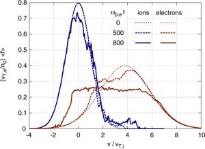
Figure 1. Snapshots of the velocity distributions in a Vlasov simulation of subcritical instability. Simulation parameters are vd/vT,i = 3.8, eφ/T ≈ 0.2 and Nx × Nv = 768 × 8192.
Download figure:
Standard image High-resolution imageFigure 2 shows the time-evolution of potential energy, normalized to thermal energy, eφ/T, for three linearly stable cases, and two linearly unstable cases. For all stable cases, we hide data for times longer than half a numerical recurrence time, TR/2 = π Nv/(10kmaxvT,e). The oscillations for vd/vT,i < 4 are due to the beating of waves with opposite phase velocities. We observe that the solutions are consistent with linear theory. Note that for drift velocities of 4.2 and 4.5, the growth rate increases before saturation. This is in contrast with the conventional wave saturation, where the growth rate decreases in time. This phenomenon was predicted and confirmed in [7]. It appears for barely unstable cases, above a threshold amplitude, for which the nonlinear growth rate overcomes the linear growth rate.

Figure 2. Time-evolution of the normalized potential energy in Vlasov simulations for small, incoherent initial perturbation, eφ/T ≈ 2 × 10⁻⁴. Linear theory is shown as dashed lines.
Download figure:
Standard image High-resolution imageThe important conclusion here, is that we observe no subcritical instability. This is in contradiction with [3], where subcritical instabilities are reported for the same parameters and vd/vT,i ⩾ 1.5, even for low-amplitude initial fluctuations with eφ/T ≪ 10−2. We scanned the parameter space of velocity drift and initial amplitude, and concluded that subcritical instabilities emerge only when the drift is very close to linear marginal stability, and the initial perturbation is relatively large. Figure 3 shows the time-evolution of normalized potential energy, for vd/vT,i = 3.8, which is only 3% below marginal stability, and for large initial amplitudes. We do observe a subcritical instability when the initial amplitude is eφ/T ≈ 0.2, but not below. For vd/vT,i = 0.5, 1.5, 2.5 or 3.0, we did not obtain any subcritical instability even for initial amplitudes as high as eφ/T ≈ 2. These results are summarized in table 1, which shows whether an incoherent ensemble of waves is nonlinearly stable (W↓) or unstable (W↑). From this table, we conclude that the nonlinear stability threshold is approximately vd/vT,i = 3.5 (vd/vd,cr = 0.89).
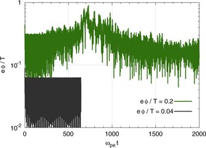
Figure 3. Time-evolution of the normalized potential energy in Vlasov simulations for vd/vT,i = 3.8 and various levels of incoherent initial perturbation.
Download figure:
Standard image High-resolution imageTable 1. Nonlinear stability. W↓ and W↑ mean decay and growth, respectively, of an initial ensemble of wave. H↓, H∼ and H↑ mean hole decay, local hole growth and global subcritical instability driven by an initial hole-like phase-space perturbation.
| vd/vd,cr | |||||||
|---|---|---|---|---|---|---|---|
| 0 | 0.38 | 0.63 | 0.76 | 0.89 | 0.97 | ||
| eφ/T | 1 | W↓, H↓ | W↓, H∼ | W↓, H↑ | W↓, H↑ | W↑, H↑ | W↑, H↑ |
| 10−1 | W↓, H↓ | W↓, H∼ | W↓, H↑ | W↓, H↑ | W↓, H↑ | W↑, H↑ | |
| 10−2 | W↓, H↓ | W↓, H∼ | W↓, H↑ | W↓, H↑ | W↓, H↑ | W↓, H↑ | |
| 10−3 | W↓, H↓ | W↓, H∼ | W↓, H↑ | W↓, H↑ | W↓, H↑ | W↓, H↑ | |
Subcritical instabilities are in many aspects qualitatively similar to linearly unstable cases. The saturation level of potential energy is similar, we observe wide particle redistribution in phase-space, especially of the electrons, turbulent heating, and significant anomalous resistivity. Figure 1 includes snapshots of ion and electron velocity distributions after the nonlinear growth for the subcritical simulation (vd/vT,i = 3.8) with high initial amplitude (eφ/T ≈ 0.2). At saturation, the electron distribution is flattened over a large range, −1 < v/vT,i < 6. The ion distribution develops a plateau around v/vT,i = 4, which is due to accumulating ion phase-space vortices.
Phase-space redistribution is associated with anomalous resistivity. We define the anomalous resistivity η as

where 〈E〉 is the spatial average of the electric field (here it is zero), and ps ≡ ∫vfs dx dv is the momentum of species s. For typical tokamak plasma conditions, n0 = 1019 m−3 and Ti = Te = 1 keV, the ion-electron collision frequency is of the order of νei ∼ 10−7ωp,e (with real mass ratio). Figure 4(a) shows the moving average (over
 of η/ηcoll where
 is a typical value of the collisional resistivity. The maximum anomalous resistivity is 4 orders of magnitude higher than typical collisional resistivity, for both subcritical and supercritical cases. In addition, ion-acoustic waves cause both ion and electron heating. We define the mean thermal energy Ts ≡ (ms/2 n0)∫(v − ps)2fs dx dv. It reduces to the temperature for spatially uniform, Boltzmann distributions. Figure 4(b) shows the moving average of the mean thermal energy perturbation δTs = Ts(t) − Ts(0). Both ion and electron thermal energies roughly double, for both subcritical and supercritical cases. These results indicate that the saturated level of turbulence, the anomalous resistivity, the turbulent heating, etc. are not directly affected by linear stability. In other words, essential nonlinear phenomena do not undergo any bifurcation at the linear stability threshold.

Figure 4. Time-evolution of (a) anomalous resistivity, normalized to
 , and (b) mean thermal energy perturbation. Three cases are shown, the simulation of figure 1 (vd/vT,i = 3.8, solid curves), a linearly unstable case (vd/vT,i = 4.2, dashed curves), and the reference case S of figure 16 (vd/vT,i = 3.0, chained curves).
Download figure:
Standard image High-resolution image3.2. PIC simulations
The simulations of [3], which are in disagreement with the above Vlasov simulations, were obtained with a full-f PIC code, with a number of particles limited by the computing power of the time. We reproduced those simulations with Np = 102 400, and indeed recovered the results of that reference, that is, subcritical growth for vd/vT,i ⩾ 1.5. Figure 5 includes one example of subcritical instability, for vd/vT,i = 2.5 and initial amplitude eφ/T ≈ 0.03. Figure 6 is a snapshot of both ion and electron phase-spaces, at ωp,et = 400. We observe several electron holes, most noticeably at (k1x, v/vT,i) = (0.9π, 3.0). We checked that particles follow trapped orbits within the latter hole.

Figure 5. Time-evolution of the normalized potential energy in PIC simulations for vd/vT,i = 2.5.
Download figure:
Standard image High-resolution image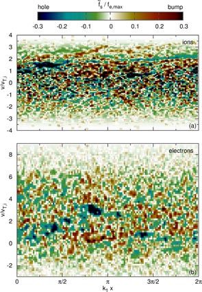
Figure 6. Snapshot at ωp,et = 400 of the phase-space in the Np = 102 400, full-f PIC simulation of figure 5 (vd/vT,i = 2.5).
Download figure:
Standard image High-resolution imageWe ran a series of such full-f PIC simulations for different values of initial drift. We define the nonlinear growth rate as
 , where
 is the depth of the deepest negative perturbation. Taking an alternative definition of the nonlinear growth rate as the growth rate of the potential energy, yields similar growth rates. This is because the potential is dominated by the largest hole, owing to the relation
 (see equation (7)). Since the growth rate depends on the amplitude, we must measure it at some fixed value of
 . We choose the same value as the reference,
 . Figure 7 shows the measured nonlinear growth rate as a function of initial drift. The data points are in agreement with simulation results of [3] (see figure 4). Besides, they are in qualitative agreement with the nonlinear instability theory of [41]. The theoretical growth rate was obtained by solving equation (99) (with the plus sign) in [41], while assuming a structure velocity v+ = vT,i (the holes have a wide range of different speeds, but v+ = vT,i is where the hole growth is expected to be the strongest), a self-binding factor b = 3 [42], a ratio
 [41], and generalized electron and ion structure lifetime as
 and τi = 2τe [3]. This theory is only meant to give an estimate of the qualitative behavior. Here we only note that the simulation data happen to agree qualitatively with the theory for this particular set of mass ratio, temperature ratio and perturbation amplitude. A careful validation of the theory is out of the scope of this paper.

Figure 7. Growth rate of electron hole. Crosses: γNL measured in full-f PIC simulations with Np = 102 400. Solid curve: nonlinear instability theory of [41].
Download figure:
Standard image High-resolution imageAlso shown is the linear growth rate for the most unstable wave-number, taking into account that the system size allows wave-numbers that are multiples of
 only. Given the agreement with theory, one is tempted to conclude that the observed instability is physical, rather than a numerical phenomenon, and that it is indeed the nonlinear ion-acoustic instability. However, these subcritical instabilities disappear (except for large initial amplitude and close to linear marginality) when the number of particles is increased or when the δf approach is adopted. Figure 5 includes time-series of potential energy in a full-f PIC simulation with Np = 224, and in a δf PIC simulation with Np = 102 400 with a similar initial amplitude (actually thrice larger at t = 0, but similar at ωp,et = 30). Both cases are stable, indicating that growth in the simulations of [3] is due to numerical noise. Indeed, we found that the initial, unperturbed velocity distribution is so noisy that it is linearly unstable.
With a number of particles as small as 102 400, the velocity distributions in full-f PIC simulations are very noisy, and only approximately Gaussian. Figure 8 shows, for vd/vT,i = 2.5, the initial ion and electron distribution functions, which were obtained by distributing the particles into 128 boxes. Substituting the distribution at Np = 102 400 into the linearized model equations, and solving the corresponding eigenvalue problem, yields a positive linear growth rate, γL/ωp,e = 0.008. Varying the number of boxes from 32 to 512, or modeling the distribution by a spline and increasing the resolution of the discretization yielded similar values, γL/ωp,e = 0.006–0.009, positive in any case. We therefore conclude that the instabilities observed in [3] were not subcritical, but linearly unstable, even when the drift was below the linear threshold for Gaussian distribution.

Figure 8. Velocity distributions at t = 0 in full-f PIC simulations.
Download figure:
Standard image High-resolution imageThe agreement between noisy simulations and theory can be explained as follows. The noisy distributions are such that, in small regions of velocity space, ∂vf0,e/me + ∂vf0,i/mi > 0. This enables waves to grow linearly from small amplitudes eφ/T ≪ 10−2, which leads to the formation of phase-space structures by particle trapping. Subsequently, these phase-space structures grow nonlinearly, in agreement with theory, but the initial state is not subcritical.
To be clear, our conclusion is not that the theory is wrong. The theory applies to the growth of a hole that is already present, not to the growth of a hole from random perturbations. To assess the nonlinear stability, we must understand what kind of initial conditions are unstable. In the following section, we address the stability of an artificial seed structure.
4. Seed structure
We have shown that subcritical instabilities can grow from an ensemble of waves, but only close to linear marginality and when the initial amplitude is large. However, it is possible to drive subcritical instabilities from much smaller initial amplitude, and even far from marginal stability, by preparing a self-trapped structure at t = 0.
Hereafter, we study the evolution of a local, negative phase-space density perturbation (hole-like) in the electron distribution, and drop the subscript e in
. The initial electron distribution is

where
 is the hole-like perturbation amplitude, vh(t) is its velocity, Δxh and Δvh(t) are its width and velocity-width, and

if |x − L/2| < Δxh/2, otherwise H(x) = 0. The initial depth
 is chosen to satisfy the trapping condition [2],

where λ is the shielding length, which is such that (kλ)−2 is the real part of the linear susceptibility. The shape of this artificial hole-like seed is arbitrary and does not correspond to maximum entropy.
Let us study in details the evolution of one case, which we label as S. It will serve here as an example of a subcritical instability. The parameters for S are vd/vT,i = 3.0, vh(0)/vT,i = 0.8, Δvh/vT,i = 0.2, and Δxh/λD = 2. Figures 9 and 10 show snapshots of both ion and electron distribution functions in the reference case S. A video, which shows the evolution of the distribution functions, their spatial averages, the normalized potential energy, and the spectrum of potential, is available (stacks.iop.org/PPCF/56/075005/mmedia). Figure 11 shows the evolution of the depth, velocity and velocity-width of the deepest hole. The reader should keep in mind that
 is defined as the depth of the deepest negative phase-space density perturbation at each instant. In other words, we do not track one single structure throughout its evolution, but rather switch to whichever structure is the deepest. Such switching is taking place between ωp,et = 1000 and 3000, where the instantaneous maximum depth alternates between different holes. In these figures, we observe two distinct phases. In the first phase, from ωp,et = 0 to 700, the initial artificial seed dominates the phase-space. In the second phase, after 700, many structures coexist and interact. Let us separate the discussion into 1. the evolution of a single hole-like perturbation in the first phase, and 2. the impacts of many phase-space structures (phase-space turbulence) in the second phase.

Figure 9. Snapshots of ion (left) and electron (right) perturbed distribution in the reference simulation S (vd/vT,i = 3.0, vh(0)/vT,i = 0.8, Δvh/vT,i = 0.2, and Δxh/λD = 2). Values of ωp,et from top to bottom are 0, 200, 500, 700 and 1000. A contour of constant fe is dashed in (i).
Download figure:
Standard image High-resolution image
Figure 10. Same as figure 9, but for later times. Values of ωp,et from top to bottom are 2000, 2500 and 3000.
Download figure:
Standard image High-resolution image
Figure 11. Time-evolution of the depth (a) and velocity (b) of the deepest negative phase-space density perturbation in Vlasov simulations in the reference case S. The velocity width is shown by error bars at ±Δvh.
Download figure:
Standard image High-resolution image4.1. Single-structure growth
Since phase-space density is conserved along particle trajectories, the center of a hole, where particles are deeply trapped, and which therefore follows particle orbits, must conserve f. Therefore, an isolated hole can grow (decay) by climbing (descending) a velocity gradient. When the gradient is positive (negative), it must accelerate (decelerate) to grow and decelerate (accelerate) to decay. In figure 11, we observe that the artificial electron seed initially grows, from ωp,et = 0 to 400, by climbing the positive velocity gradient, thereby accelerating from vh/vT,i = 0.8 to 3.0. The growth stops when the structure reaches the top of the electron distribution (vh = vd). Then, from ωp,et = 0 to 400, it decays by descending the velocity gradient, while still accelerating. It decays until it reaches a velocity v such that
 . Before this final velocity is reached, however, the diagnostic switches to other holes, which are then deeper than the initial seed. It is these new holes that drive the nonlinear instability at later times. This process is described in the next section, 4.2.
Whether an artificial hole-like seed initially grows or not depends on both its characteristics and the plasma drift velocity. Figure 12 shows the evolution of an electron hole-like seed, initially located in the region of strong overlap between ion and electron distributions, for various initial conditions. The ratio Δxh/Δvh = 20/ωp,e is arbitrary. For vd = 0 (figure 12(a)), we observe that all seeds (for the shapes and sizes we tested, as listed in the legend of figure 12) are damped. This is expected since in this configuration, there is no free-energy. Note that in this configuration, an isolated hole must accelerate (descend the velocity gradient) to decay. Trapped particles accelerate with the hole. Thus, a phase-space structure can drive transient velocity-space particle transport, even as it decays.

Figure 12. Time-evolution of the depth of the deepest electron phase-space perturbation
 in Vlasov simulations with an initial electron seed with Δxh/Δvh = 20/ωp,e. The initial drift vd/vT,i is (a) 0.0, (b) 1.5 and (c) 3.0. The reference simulation is marked by S in (c).
Download figure:
Standard image High-resolution imageFor vd/vT,i = 3.0 (figure 12(c)), which is relatively close to linear threshold (vd = 0.76 vd,cr), all seeds (for the shapes and sizes we tested) initially grow. The evolution is similar to the reference case S. For vd/vT,i = 2.5, results are qualitatively similar and are not shown here.
For an intermediate value of drift, vd/vT,i = 1.5 (figure 12(b)), which is far from the linear threshold (vd = 0.38vd,cr), the hole growth and subsequent decay depends on its size and location. When they are located in the velocity-region of strong overlap between ion and electrons, holes seem to grow more easily. This is consistent with the underlying growth mechanism (local momentum exchange between ions, electrons and waves) and with the predicted theoretical growth rate of an isolated hole. The hole growth is expected to be of the order of
 , where ωb is the bounce frequency of a particle deeply trapped in the hole [32]. However, in all cases, the hole eventually decays and no other phase-space structure is generated. Whether a hole with a different shape can or cannot trigger phase-space turbulence remains an open question, since we have studied only six cases.
In (figure 12(b)), we observe that holes initially decay for a while before starting to grow. The reason may be that the shape of the artificial initial seed is not optimal for growth. This hypothesis is supported by the following analysis. Figure 13 compares two cases, where Δvh(0) is fixed to 0.2 vT,i, but Δxh(0) differs. If Δxh(0)/λD = 2, which corresponds to a ratio
 , the ratio Δxh(t)/Δvh(t) executes damped oscillations around a value of
 , until it stabilizes. Then the hole starts its nonlinear growth. If Δxh(0)/λD = 5, which corresponds to a ratio
 , the hole starts to grow almost straightaway, suggesting that its shape is closer to the optimal shape for nonlinear growth.

Figure 13. Time-evolution of (a) the height of the largest electron hole and (b) the ratio Δxh/Δvh in Vlasov simulations with an initial electron hole with Δvh(0)/vT,i = 0.2, for vd/vT,i = 1.5 and vh(0)/vT,i = 0.4.
Download figure:
Standard image High-resolution image4.2. Phase-space turbulence
For a velocity drift vd/vT,i = 1.5, we mentioned that, although the hole initially grows, it eventually decays and no other phase-space structure is generated. In such cases, we observe that the electric potential does not increase. The velocity redistribution is negligible (〈δfs〉/fs,0 < 10%), the mean thermal energies are constants (δTs/Ts < 0.1%), and the anomalous resistivity is small (η/ηcoll < 500). Thus, the nonlinear growth of one isolated hole is observed without system-wide instability. We refer to this situation as local hole growth.
This local hole growth contrasts with the global subcritical instability observed e.g. for the reference case S. Figure 14 shows snapshots of the velocity distributions in the latter case. We observe wide particle redistribution between
 and
and
 , which is after the initial hole has decayed, and during the growth of the new holes. We can check that particles are indeed trapped into the self-emerging structures. Figure 15 shows the velocity vp of a test electron, which is deeply trapped by a hole formed around
 . The central velocity of the hole vh is estimated by tracking the local minimum of f. The velocity of the test electron in the framework of the hole, vp − vh, is shown to oscillate around zero, which indicate that particles follow trapped orbits in phase-space, in the reference-frame of the structure. The bounce frequency is measured from the time-trace of vp − vh as ωb ≈ 0.15ωp,e. Another way to estimate the bounce frequency is to measure the local maximum φ0 of the electric potential, and the spatial extent Δxh of the negative perturbation. The bounce frequency is then given by
 , with kh = 2π/Δxh. This method also yields ωb ≈ 0.15ωp,e for the same hole. The oscillation is quasi-periodic from
 to
to
 . At t2, the hole appears to be sheared by the tidal forces exerted by a neighboring, larger hole. The lifetime of the hole is thus estimated as τc = t2 − t1 = 430. The Kubo number in the region of phase-space within this hole is K = ωbτc/(2π) ≈ 10. Repeating this analysis for other holes among the largest ones, we found Kubo numbers in the range K ≈ 3–20. This confirms that the simulation is in a regime of large Kubo number. The merging of holes reduces their lifetime. However, merging is rare enough that particles bounce many times during the life of most large holes.

Figure 14. Snapshots of velocity distributions, in the reference simulation S.
Download figure:
Standard image High-resolution image
Figure 15. Time-evolution of the velocity vp of a test particle (electron) trapped in a hole with central velocity vh(t), in the reference simulation S.
Download figure:
Standard image High-resolution imageFigure 16 shows the moving average (over
of the potential energy time-series in three cases, including the reference case S, for vh/vT,i = 0.8. We observe that the potential energy grows to eφ/T ∼ 0.3, which is of the same order as the saturated potential in linearly unstable cases. In the reference case S, we see a clear difference between the first phase (t = 0 − 700) and the second phase (t = 700 − 2000). In the first phase, a single hole develops (as seen in figures 9(c), (e) and (g)), and although the field energy grows, it is only transiently. The field energy then decays back to a value close to the initial perturbation. In the second phase, where multiple holes develop (as seen in figure 9(i) and (b)), the field energy grows to eφ/T ∼ 0.3 before relaxing to eφ/T ∼ 0.1, thereby driving a global subcritical instability. Therefore, for a given initial field energy, phase-space turbulence (multiple interacting holes) is more efficient than a single hole to drive the instability.

Figure 16. Time-evolution of the normalized potential energy in Vlasov simulations with an initial electron hole, for vd/vT,i = 3.0, vh/vT,i = 0.8, Δxh/Δvh = 20/ωp,e and varying hole velocity-width. The reference simulation is marked by S.
Download figure:
Standard image High-resolution image
Figure 4 includes the time-evolution of anomalous resistivity and perturbed mean thermal energies for the reference case S. We observe large anomalous resistivity and turbulent heating, qualitatively similar to the cases with an initial ensemble of waves. These subcritical instabilities occur relatively far from marginal stability, even when the initial potential energy is as low as eφ/T ∼ 10−2. This is in sharp contrast with the case where the initial perturbation is a collection of waves. In other words, phase-space structures, even with non-optimal shapes, are much more efficient than coherent waves for driving nonlinear instabilities.
To summarize, we observe that many holes, even small, but when scattered in phase-space, can drive global subcritical instabilities. In contrast, one single hole, even a large one, can evolve while leaving most of the phase-space intact, without system-wide instability (without significant potential energy growth, redistribution, heating or anomalous resistivity). One single hole can drive instabilities indirectly though, by triggering the formation of many smaller holes in its wake. This process is detailed as follows. As can be seen in figure 9, as the initial, artificial hole accelerates within the region vh < vd, its depth increases (along with its width in velocity). This increase in depth is due to the trapping of additional particles. This leaves a trail of negative phase-space density perturbations in the region vh < vd (see figures 9(c) or (e)). Then, as the hole enters the region vh > vd, its width in velocity decreases, and de-trapping occurs. This, in turn, leaves a trail of positive phase-space density perturbation in the region vh > vd (see figure 9(g)). In analogy to self-gravitating matter organizing into hierarchical structures via the mechanism of Jeans collapse, negative phase-space density perturbations have a natural propensity to coalesce [8, 43]. The negative trail bunches into a collection of small holes, scattered in phase-space (see figures 9(g) and (i)). The turbulent interaction of these many holes (phase-space turbulence), is shown in figure 10. From our analysis, we conclude that phase-space turbulence is a very efficient source of particle-transport in velocity space (or redistribution), turbulent heating and anomalous resistivity.
The above nonlinear stability analysis of phase-space holes is summarized in table 1, which shows whether a hole decays (H↓), grows but then decays without triggering system-wide electron redistribution (local growth, H∼) or grows and trigger such redistribution (global subcritical instability, H↑). From this table, we conclude that the nonlinear stability threshold with an initial hole in terms of vd/vT,i is between 1.5 and 2.5.
To study the effect of larger wave-lengths, we ran many of the simulations above with a quadrupled system size, allowing wave-numbers as small as
 . We did not find any qualitative difference in the results.
Recently, we have discovered a new kind of self-organized structure, called a phase-space jet [35]. In figure 9(i), we superimposed a dashed curve of constant fe (not constant
 , which spans a velocity range 3vT,i = 1.5vT,e. This structure is highly anisotropic. It has a lifetime
 , which is comparable to the average time it takes a particle to change its velocity by vT,e,
 . Thus it is a phase-space jet, which can facilitate electron redistribution. We conclude that phase-space jets are spontaneously created in subcritical (as well as linearly unstable) conditions.
5. Discussion
We now turn to a discussion of experimental scenarios, the effect of collisions, of a magnetic field and of the mass ratio. The purpose of this section is not only to clarify caveats, but also to stimulate further studies, and is more of a speculative flavor.
5.1. Experimental scenarios
Our numerical analysis clarify the process of phase-space structures formation. If the system is linearly unstable, a turbulent state can be reached, in which particles are randomly scattered, leading to fine-grain structures that act as seeds. If the system is linearly stable, we can speculate that at least four routes to instability are possible. The first route was demonstrated in figure 3. It corresponds to the growth from random fluctuations. This route is limited to an initial barely stable equilibrium and requires large amplitude perturbations. The initial perturbation (e.g. thermal noise) can be seen as an ensemble of waves, which will trap particles and form seed structures that can grow nonlinearly. The second route was demonstrated in figure 12(c). It corresponds to the growth of a single hole. Such holes may be externally driven by the experimental setup or by physical processes that are not included in this model. As we have seen, a single hole may or may not lead to phase-space turbulence. We speculate the existence of a third route, which would be a transition from supercritical to subcritical instability on a fluid time-scale. Fluid parameters of the background plasma such as fluid velocities or temperatures may evolve, on a slow time-scale, due to processes that are not included in this model, such as an applied electric field, external heating, or other magneto-hydrodynamic instabilities. This may lead to a transition from a linearly unstable system to a linearly stable state. Phase-space turbulence that originates from linearly-driven seeds should be able to survive this transition. A fourth route was demonstrated by NGuyen [44, 45]. It is a transition from supercritical to metastable (subcritical steady-state) on a kinetic time-scale. As the wave grows linearly, the ion resonance width increases. Eventually, trapped ions absorb wave energy at a rate for which the total nonlinear growth rate vanishes. Such process can result in a metastable steady-state, where phase-space structures may be continuously created and dissipated. These scenarios are summarized in table 2.
Table 2. Scenarios that may lead to a turbulent state with phase-space granulation. Here, IP is short for initial perturbation, and transition refers to transition from supercritical to subcritical conditions.
| Scenario | Linearly stable | Seed PS structure(s) | Requires high-amplitude IP | Sensitive to details of IP |
|---|---|---|---|---|
| Supercritical instability | No | Trapping islands | No | No |
| Marginal stability | Barely | Thermal noise | Yes | Yes |
| External drive | Yes | Externally-driven hole | Yes | No |
| Fluid transition | Yes | Pre-existing structures | No | No |
| Kinetic transition | Yes | Pre-existing structures | No | No |
5.2. Effect of collisions
This work is concerned with collisionless plasma, but even small collisions can have qualitative effects on the nonlinear evolution of wave-particle interactions [12, 46]. If a collision operator that tries to recover a Gaussian distribution is introduced, we expect to find regimes of intermittent, rather than transient, turbulence. This is a speculation, based on the known effects of collisions on phase-space structures in the bump-on-tail instability.
5.3. Effect of the mass ratio
Phase-space holes in pair plasmas with small mass ratios are ubiquitous in semiconductors and space [47]. However, the small mass ratio mi/me = 4 adopted in this work brings the question of applicability of our findings to the most common hydrogen-ion plasma. In the opposite limit of an electron–oxygen-ion plasma with mass ratio mi/me = 29 500, a single electron hole remains stationary for a hundred
 , until an ion density cavity is formed [48]. Whether phase-space turbulence and subcritical instabilities develop or not on a ion kinetic time-scale
 in large mass-ratio plasma remains an open question. Moreover for larger mass ratio, the phase-space turbulence will probably not affect the ion distribution and its mean thermal energy.
5.4. Effect of a magnetic field
While in this work we focused on current-driven ion-acoustic instability in unmagnetized plasmas, similar scenarios can be developed for magnetized plasmas. Formation of a single phase-space structure is reported in [25]. In that paper, it was shown that a drift-hole extracts free energy more efficiently than linear waves do. The turbulent case with many structures is discussed in [15]. In this work it was shown that in trapped-ion resonance driven, ion temperature gradient instability, transport is determined, not by quasi-linear turbulent diffusion, but rather by dynamical frictions exerted on turbulent trapped-ion granulations. More recently, it was shown that both a coherent drift-hole and an ensemble of granulations can interact with zonal flows [20, 49, 50]. The impact of zonal flows on transport driven by trapped-ion granulations was formulated as a part of dynamical friction [51]. In magnetized space plasmas, phase-space turbulence and jets are promising candidates mediators of magnetic reconnection via anomalous resistivity.
6. Summary
Accurate Vlasov simulations of subcritical two-species plasma have shown that subcritical excitation of the ion-acoustic instability is much more sensitive to initial perturbation than was reported in the existing literature. If, on the one hand, the initial perturbation is an ensemble of wave, a system with finite ion–electron relative drift does not evolve if it is linearly stable. However, if it is close to marginal stability, and the initial perturbation is very large, the system absorbs the wave energy to form phase-space structures. These structures allow the system to relax by transporting trapped particles throughout the phase-space. In the final stage, a velocity plateau is formed in the electron distribution. If, on the other hand, the system has an initial coherent structure, then it evolves even for small drift velocities. The stability of the initial structure is much more akin to the BGK stability problem. When the initial structure is unstable, the system may or may not ultimately relax into a velocity plateau, depending on the drift velocity and the parameters of the initial structure.
Table 1 summarizes our nonlinear stability analysis, showing, in the parameter space of initial velocity-drift and potential energy, where we have observed global subcritical instability (↑), from either an ensemble of waves (W) or an artificial hole (H). These results are in disagreement with earlier numerical works. In fact, earlier simulations were so noisy that the initial distribution was linearly unstable. Thus, this paper reports the first simulation of subcritical ion-acoustic instability.
When the velocity drift is finite, a single electron phase-space hole can grow nonlinearly by climbing the velocity gradient. After it reaches the top of the electron distribution v0,e, it decays while still accelerating. This process leaves a trail of negative fe perturbations in the v < v0,e half of the phase-space, and a trail of positive perturbation in the other, v > v0,e, half. Negative perturbations have a natural propensity to coalesce, and form many holes. This process can overcome ion Landau damping when vd > 0.5vd,cr (roughly). When many holes are formed, a large region of phase-space becomes turbulent, and individual holes lose their identity, and so resemble granulations [52]. Phase-space turbulence is very effective in flattening the electron distribution, heating both ions and electrons, and driving anomalous resistivity [17].
We have shown the existence of phase-space jets in states resulting from subcritical instabilities. Jets are studied in a separate paper [35]. They are elongated closed contours of constant f, which coexist with holes. These jets facilitate particle redistribution and drive anomalous resistivity.
Acknowledgments
The authors are grateful for stimulating discussions with K Itoh, S-I Itoh, C Watt, C Nguyen, Y Idomura, X Garbet and the participants in the 2009, 2011 and 2013 Festival de Théorie. This work was supported by grants-in-aid for scientific research of JSPS, Japan (21224014, 25887041), by the collaboration program of the RIAM of Kyushu University and Asada Science Foundation, by the WCI Program of the NRF of Korea funded by the Ministry of Education, Science and Technology of Korea [WCI 2009-001], and by CMTFO via U.S. DoE Grant No. DE-FG02-04ER54738. Computations were performed on the XT and SX systems at Kyushu University.