
Abstract
A new ion cyclotron resonance frequency (ICRF) modulation technique has been developed and exploited at ASDEX Upgrade for obtaining time perturbed boron density signals. Square wave modulation of the ICRF heating power results in a periodic modulation of the boron density in the edge, which propagates inward. From this time perturbed boron density signal, the boron diffusivity and convection in the radial transport equation are individually determined. This task is done by solving an inverse problem by a quasi-Newton method. This implemented framework has been verified with the Method of Manufactured Solutions and benchmarked with the transport code STRAHL. The experimental transport coefficients are compared with neoclassical calculations with the code NEO and gyrokinetic simulations with the code GKW. The neoclassical diffusivity is well below the experimental one. The comparison to gyrokinetic theory shows a good agreement in the diffusivity, but the theoretical convection predicts a more peaked boron density profile than measured in the experiment.
Export citation and abstract BibTeX RIS

Original content from this work may be used under the terms of the Creative Commons Attribution 3.0 licence. Any further distribution of this work must maintain attribution to the author(s) and the title of the work, journal citation and DOI.
1. Introduction
Impurities in fusion plasmas arise from many different sources including the erosion and sputtering of materials from plasma facing components, the intentional injection of impurities via gas puffing, pellets, or laser blow-offs for divertor cooling, core radiation control, or physics studies, and the production of helium from the fusion process itself. The plasma performance is highly affected by the impurity concentration and, to achieve a stable burning plasma scenario in future reactors, the build up of impurities in the plasma core must be controlled. Therefore, a fundamental understanding of the mechanisms behind impurity transport in fusion plasmas as well as identifying the engineering parameters with which the transport can be controlled are of great importance. In the past years impurity transport studies of both low-Z and high-Z impurities have been conducted in a broad variety of plasma conditions in several different tokamaks around the world. The most common ways of injecting impurities for transport studies are with gas puffing [1–5] or laser blow-offs [6–9].
Impurity transport perpendicular to flux surfaces can be described by diffusion and convection. This can be formulated in the radial transport equation [10]
In equation (1),  is the impurity density for an impurity species Z, D(r) is the diffusion coefficient, v(r) is the convection or drift velocity, and s(t) is the impurity density boundary condition at the edge, rmax. This equation is written in cylindrical coordinates, with r being the radial coordinate, which has been chosen such that
  , where V is the volume within the flux surface and
  is the major radius of the magnetic axis [11]. With this choice the flux surfaces are transformed into circles conserving the plasma volume [11]. Note that in equation (1) the transport coefficients have no dependence on the poloidal angle and, therefore, represent flux surface averaged quantities [12]. In tokamak plasmas, magnetic flux surfaces are in general not circular, but are approximately elliptic. This ellipticity is neglected in the analysis. However, it is possible to estimate the impact of the ellipticity on the deduced transport coefficients by calculating the missing factor of
  [13]. Including this factor gives a modification to the particle flux and, thus, to the transport coefficients of 2%–3% in the center, 7%–8% at mid-radius, and up to 20% at ρtor ∼ 0.7. These small corrections are well within the experimental error bars.
If the impurity density profile is constant in time, that is  , equation (1) reduces to the steady-state equation
Suppose a D and v are found that satisfy equation (2). Then it is straight-forward to see that  and
and  , where C is a positive constant, is also a solution to equation (2). Hence, from only the steady-state equation (2), the transport coefficients cannot be uniquely determined. To disentangle v and D from one another, one needs to measure the temporal evolution of the impurity density profiles after a perturbation, e.g. during a modulation of the impurity source at the plasma edge.
In this work, a novel method of inducing a time perturbed boron density at ASDEX Upgrade (AUG) has been developed and utilized to uniquely determine the transport coefficients D and v in AUG H-mode plasmas. This method combines the advantages of a transient transport analysis performed on modulated signals over many periods, as often applied for heat transport studies, with the high radial resolution enabled by charge exchange recombination spectroscopy (CXRS), which, at AUG has so far only been used for the measurement of impurity density profiles for transport analysis in stationary conditions [10, 14]. The use of CXRS limits the applicability of the method to sufficiently light impurities. This, however, does not reduce the physics interest of this approach, which, as it will be shown in the present application, delivers accurate, highly radially resolved, separated measurements of the boron transport coefficients. The importance of determining the diffusion D and drift velocity v separately can be readily understood considering that this also allows more complete comparisons with the theoretical predictions of impurity transport models. This lends itself directely to the goal of increasing our confidence in the prediction of the diffusion of helium, which is a critical parameter in determining the impact of the central helium source produced by fusion reactions. Moreover, accurate investigations dedicated to light impurities are of critical importance in the validation of impurity turbulent transport models. This is an important element in the prediction of the impurity density profiles in a fusion reactor plasma, also for highly charged impurities. In fact, in present experiments the transport of heavy impurities is much more dominated by the neoclassical convection [15], in contrast to light impurities which are more dominated by turbulent transport [2, 3, 5, 14]. At the very low collisionalities of a reactor, however, the role of turbulent transport can be expected to become significantly more important also for heavy impurities [16].
This paper is organized as follows: section 2 describes the new modulation method as well as how the transport coefficients can be deduced from this modulation signal. In section 3 the validation of the method as well as its uncertainties are discussed. The first experimental results with an initial comparison to neoclassical and gyrokinetic theory are presented in section 4. This is followed by a conclusion in section 5.
2. Methodology
2.1. Boron density modulation with ICRF
The experiments in this work were conducted at AUG, which is a medium-sized, tungsten walled, divertor tokamak situated at the Max-Planck Institute for Plasma Physics in Garching, Germany [17]. The major and minor radii of the machine are 1.65 m and 0.5 m, respectively, and it is equipped with a comprehensive suite of diagnostics as well as flexible and powerful heating systems including neutral beam injection (NBI), electron cyclotron resonance heating (ECRH), and ion cyclotron resonance frequency (ICRF) heating [18]. At AUG, it was observed that a modulation of the power of the boron- and tungsten-coated ICRF antennas results in a modulation of the boron density in the plasma. This can be clearly seen in figure 1, where the ICRF heating power is presented in blue and the resultant boron modulation signal in red for one CXRS channel at ρtor = 0.76. The boron modulation is stronger at the edge than in the core and the edge also responds more quickly than the core to the change in the ICRF heating power, which indicates a change in the boron source from the edge plasma rather than a change in core transport, as the measurement of the boron influx at the limiters also increases when the power of the antennas is modulated. Therefore, this technique can be used for core boron transport studies. The exploration of this possibility is the subject of this work.

Figure 1. ICRF heating power modulation with a frequency of 8.33 Hz (blue) and the resultant modulation of the boron density at ρtor = 0.76 (red).
Download figure:
Standard image High-resolution imageIt was discovered already in the 1980s that the operation of ICRF antennas can cause an increased influx of metallic impurities [19, 20], which arises due to the RF sheath potentials in the Faraday screen gaps [21, 22]. The ICRF concept in this work is similar to the work in [23], in which the tungsten transport at the edge was studied by modulating the power of the ICRF antennas. The ICRF heating system at AUG has been updated and is now comprised of four antennas in pairs of two: two 2-strap boron-coated and two 3-strap tungsten-coated antennas [24]. In this study, all the ICRF antennas are operated in phase and the ICRF heating scheme used is the hydrogen minority heating with a frequency of the ICRF generators of 36.5 MHz.
A feasibility study was conducted to better understand the boron source and if the technique can be used for transport studies. At AUG, boron is considered to be an intrinsic impurity due to the regularly performed boronizations, during which the vessel wall is covered with a thin layer of boron [25, 26]. It has been observed that the boron modulation signal is strongest when the experiments are performed in a freshly boronized machine. This suggests that the ICRF heating power modulation affects the boron coating on the antennas which originates from the boronization and not the boron of the antenna itself. This hypothesis is strengthened by the fact that a strong modulation signal is also achieved when only modulating the tungsten-coated ICRF antennas. Furthermore, only a modulation of the ICRF antennas have an impact on the boron density, since attempts at modulating the ECRH at various power levels did not result in a boron modulation. To enable boron CXRS measurements of good quality at AUG, a minimum of 2.5 MW of NBI power is necessary when performing these experiments. The feasibility study also demonstrated that this technique is applicable in a broad variety of H-mode, lower single null plasma conditions, although only one experimental dataset is shown in this paper. Apart from that the method is insensitive to the current, magnetic field, and plasma parameters. So far, the ICRF modulation has only been observed to affect the boron content in the plasma; helium, carbon, and nitrogen show no modulation behavior. On the other hand, the concentrations of these impurities were very low, making a possible modulation perhaps beyond detection. All in all, this method may be applicable in other machines which have carbon walls or also utilize boronization as a wall conditioning technique.
A requirement for the feasibility of this technique is a steady plasma background, which means keeping the electron density, the ion, and the electron temperatures constant such that the transport coefficients D and v are not time-dependent during the modulation. From the feasibility experiments it is clear that the amplitude of the measured boron density modulation scales with the ICRF heating power, but increasing the ICRF heating power also causes a bigger modulation of the ion and electron temperatures. Therefore, one has to choose an ICRF power level at which a clear modulation of the boron density is observed, while the modulations of the other quantities are kept as low as possible. From the study it was concluded that a power level of ∼1 MW of ICRF heating is sufficient to modulate the boron density up to 10% at the edge while keeping the modulation of the ion and electron temperatures to less than 1%–4%. Different modulation frequencies were tested and also here a balance between a clear boron modulation signal and the perturbation to the plasma background has to be maintained. The modulation frequency chosen for the ICRF heating power is 8–10 Hz and this frequency is directly translated to the perturbation seen in the boron density, which is clearly visible in figure 1.
2.2. Measuring the boron density with CXRS
At AUG two core CXRS systems regularly measure the boron content in the plasma. In total these systems have 72 lines-of-sight (LOS) and a typical integration time of 10 ms [27, 28]. The two core systems are located on opposite sides of the torus and, hence, view two different NBI sources, with beam energies of 60 keV (box I) and 93 keV (box II), respectively. The spatial and maximal temporal resolution of the system utilizing the 60 keV beam are 1.0–2.5 cm and 3.5 ms [27], while for the system utilizing the 93 keV beam they are 1–1.5 cm and 2.5 ms [28]. However, the systems are often signal limited to longer integration times. The experimental data shown in this paper is from the core system viewing the 93 keV beam (box II), but as a consistency check the density profiles are cross-checked and validated against the other core system viewing the 60 keV beam. The measurements presented in this paper were performed with an integration time of 10 ms.
The CXRS diagnostics measure the spectral line emission from the charge exchange interaction of the the neutral beam particles with the impurities in the plasma [29, 30]. The plasma rotation can be deduced from the measured Doppler shift and the ion temperature from the Doppler broadening of the spectral line. From the measured line intensities ICX,Z the impurity density nZ can be calculated in the following way:
where  is the effective CX emission rate coefficient for a given spectral line,
  are the neutral atoms from the beam for a given energy component i and a given excited state j of the beam. The calculation of the impurity density has been performed with the in-house CHICA code, which stands for charge exchange impurity concentration analysis. To calculate the impurity density, CHICA takes the electron density, electron temperature, ion temperature, the measured CXRS line intensity, and the plasma equilibrium as inputs. The resultant impurity density profile depends strongly on these input profiles, especially the electron density, hence they have to be well known. Another important factor for the calculations is the geometry of the beams. The beam geometries have been constrained using beam emission spectroscopy (BES) measurements with different LOS as well as thermal images of the beam impact points on the inner wall. The cross-check of the calculated impurity density profiles between the CXRS systems on box I and box II, which have different geometries and energy components, provides confirmation that the beam geometries are correctly calculated. Differences in absolute magnitude of 10%–20% are often seen between the diagnostics and are attributed to calibration uncertainties and unavoidable deterioration of the in-vessel optical components during the experimental campaign. However, for determining the transport coefficients it is the gradient, e.g. the profile shape, that is important and, as can be seen in figure 2 and [28], both systems reproduce the same profile shapes. Note that in figure 2, a correction factor of 0.88 was applied to the density profile of the NBI box I CXRS system to match the absolute value of the impurity density profiles. Linear fits of the two datasets in the radial window ρtor = 0.4–0.6 are performed and the correction factor is determined from the ratio of the radial averages of the two linear fits. This is a standard method for combining the two datasets.

Figure 2. Steady-state boron density profile for the two CXRS core diagnostics. A correction factor of 0.88 has been applied to the NBI box 1 CXRS system to match the absolute value of the boron density profiles.
Download figure:
Standard image High-resolution imageThe neutral beam density n0 in equation (3) can be measured with BES or calculated with various beam attenuation codes. In this work, a beam attenuation code has been utilized. The beam has three different energy components as well as a beam halo making i = 1, 2, 3, 4 in equation (3). Furthermore, the beam and the beam halo can be in different excited states j. The beam halo is a cloud of deuterium neutrals around the injected neutral beam, which are produced from charge exchange interactions between the injected neutral particles and the thermal plasma deuterium ions. The effective charge exchange emission rates  for a given spectral line are derived from the charge exchange cross-sections found in the ADAS database [31]. The effective rate
  is obtained by integrating σv over the velocity space of the beam neutrals and the impurity. The product of the neutral beam density n0 and effective charge exchange emission rate
  is integrated along the LOS and then summed over the different energy components and excited states. Note that in equation (3) the boron density is assumed to be constant along the intersection of the LOS and the neutral beam volume. This assumption is well met in the plasma core where the gradient lengths are small, but is not valid for the CXRS LOS that intersect in the edge pedestal inside of the beam volume. This is the case for the outermost LOS of both core systems (ρtor > 0.85). For these LOS, special analysis is required that has not been performed here and to avoid any effect of uncertain gradient on the profiles, the analysis region is restricted to ρtor < 0.70.
2.3. Numerical scheme
Solving equation (1) for the impurity density nZ given a D and v is called the forward problem. However, the situation at hand is the opposite: the measured boron density nB is known and the corresponding D and v profiles should be deduced. This is the inverse problem. This task, unlike the simple forward problem, is non-trivial since the problem itself is ill-posed, thus small errors in the measured data are greatly amplified in the solution. One way of regularizing the problem is to impose smooth D and v profiles. The boron density nB is measured at discrete radial locations  and time points
  , where rl denotes the radial and tk the time measurement positions. tk depend on the integration time of the CXRS diagnostic and rl on the geometry of the LOSs and their intersection volumes with the NBI. This yields the measured data points
  , such that there is no continuous representation of nB(r, t) available from which the v and D profiles can be calculated directly as in [32]. Therefore, smooth v and D profiles have to be found such that the resulting simulated local densities nS evaluated at the measurement points nS(rl, tk) are in good agreement with the measured data
  . This inverse problem can be cast in the formalism of a minimization. By inserting some initial D and v profiles in equation (1) a forward calculation is performed yielding a simulated density nS(r, t). The simulated density is evaluated at the discrete measurement points resulting in nS(rl, tk) such that the difference between the measured and simulated density at the respective points can be expressed by
  . By varying the input D and v profiles a new value of
  is obtained and this process is iterated until a minimum of the difference is found. In this way, the D and v profiles corresponding to the measured boron density nBl,k is acquired. This minimization procedure can mathematically be written as:
where σBl, k = σB (rl, tk) are the standard deviations of the densities at the measurement points rl and tk. Since the measured boron signal is periodic (see figure 1), a robust ansatz for the reconstructed density nS(r, t) as well as the boundary condition s(t) which fits the measured data particularly well is
In equation (5), n0 is the steady-state density and ω = 2πf, where f is the frequency of the modulation. The boron source term s(t) is assumed to have the same time dependence as the density nS. This ansatz is used when solving the inverse problem (4) and inserting the ansatz in equation (4) yields
By also inserting the ansatz in the radial transport equation (1), three equations are obtained: one for the steady-state n0(r)

and two for the modulation part 


Inserting the boundary condition s(r) in the transport equations yields


where rmax is the last data point of the experimental data. Finally, the Neumann boundary conditions for D and v, which resolve the singularity at r = 0, can be expressed as follows:


Equations (6)–(14) represent the complete mathematical description of the minimization problem. The model can thus be reduced to the steady-state and the modulation at the frequency ω, which corresponds to a Fourier transform in time at the modulation frequency. Thus, no time discretization is necessary.
In this work, equation (4) is solved with sequential least squares programming [33], which is a quasi-Newton method, yielding the reconstructed density nS by solving equation (1) for various D and v profiles as well as the source term s, which is composed of the coefficients s0, a0, and b0. The implementation of the problem has been set up in Python using the Scipy minimization library [34]. Second order finite differences are used for solving the transport equation. The D and v profiles are represented with arbitrary order B-splines, which enforce smoothness of the solution and is therefore a way of applying a regularization to the ill-posed problem. The minimization is thus performed over the B-spline knots of D and v as well as the coefficients s0, a0, and b0. An example of the measured (left) and reconstructed (right) boron density is presented in figure 3. This shows very good agreement. This becomes even clearer when studying the left-hand side of figure 4, which displays the difference between the simulated and measured boron density  . No additional modulation at the modulation frequency of 8.33 Hz or any other frequencies can be seen and hence, the ansatz from equation (5) is, for this problem, very well suited. This claim is further confirmed by computing a Fourier decomposition of the measured boron density nB at ρtor = 0.21 (blue curve on the right-hand side of figure 4), which only displays a peak at the modulation frequency at 8.33 Hz, hence no higher harmonics are present in the central region of the plasma. In orange the same quantity at
  is shown. At this location near the plasma edge, additional smaller peaks are visible at the second and third harmonics, indicated by the black dash-dotted lines. These peaks are, however, one order of magnitude smaller than the peak at the first harmonics, i.e. 8.33 Hz, and barely distinguishable from the noise. Furthermore, the Fourier decompositions of the differences between the simulated and measured boron density
  at
at  and
and  are plotted with dashed green and red lines, respectively, and this quantity shows no additional frequency peaks outside of the noise.

Figure 3. Left: contour plot of the measured boron density. Right: contour plot of the reconstructed boron density. Note that the two plots have the same colorbar.
Download figure:
Standard image High-resolution image
Figure 4. Left: contour plot of the difference between the simulated and measured boron density  . Right: Fourier decomposition of the measured boron density nB at
  in solid blue and at
  in solid orange as well as the difference
  at
at  in dashed green and at
  in dashed red. Lines indicating the first, second, and third harmonics in dash-dotted black.
Download figure:
Standard image High-resolution imageIn the dataset presented here, sawteeth are present with a frequency of 16 Hz and an inversion radius of ρtor ∼ 0.25. That corresponds to ∼1.6 sawtooth cycle for every CXRS integration time. The experimental data inside of ρtor < 0.25 is, hence, a sawtooth average, and therefore, the sawtooth frequency cannot be seen in the right plot of figure 4.
3. Method validation and uncertainties
3.1. Method validation
With the new ICRF modulation technique multiple modulation cycles can be measured and analyzed together in an otherwise constant background plasma, see figure 3. This is a big advantage compared to other techniques such as laser blow-off and gas puffing, which commonly determine the transport coefficients by analyzing only one single cycle, for example, one individual laser blow-off. The method presented here reduces the relative noise and has a lower statistical uncertainty.
Before using the numerical simulation tool to predict the transport coefficients, it is important to build trust in its reliability and make sure the solver has been implemented correctly. This can be done by checking whether the simulation tool accurately reproduces an analytical solution. This approach is called the method of manufactured solutions [35, 36]. The procedure is straight-forward: suppose the D and v profiles have been found. The transport equation can then be solved analytically for the steady-state n0(r) by integrating equation (2) from r to rmax:
Expanding both sides yields:
By inserting analytical D and v profiles in equation (17), an analytical expression for n0(r) can be calculated. The analytical n0(r) is compared to the the n0(r) obtained by inserting the same analytical D and v profiles into the second order finite difference solver for the transport equation. If the two different approaches give the same n0(r), the radial transport solver has been correctly implemented. This test was performed and the normalized analytical steady-state n0(r) (blue) and the steady-state n0(r) obtained from the solver (orange) are presented in figure 5. The agreement is perfect and it can, thus, be concluded that the radial transport solver has been correctly implemented.

Figure 5. Code verification with the the method of manufactured solutions. The blue curve represents the normalized analytically calculated steady-state n0 and the orange curve is the steady-state acquired from our radial transport solver.
Download figure:
Standard image High-resolution imageTo investigate what features can be resolved in the transport coefficient profiles with the AUG CXRS diagnostics, further method validation was performed. Synthetic D and v profiles were given to the radial transport solver and the steady-state n0 density, phase and amplitude profiles were calculated (see section 4 on how the phase and amplitude are calculated). In the following examples, the frequency of the modulation was 10 Hz.
First, the D and v profiles (blue lines called True in figure 6) were scaled with a factor of 1.3 (dashed orange lines in figure 6). Additionally in red, example experimental data points with typical error bars are plotted for the steady-state density, phase, and amplitude to display what kind of features we are able to measure with our CXRS systems. It should be noted that our CXRS diagnostic has three times as many data points, but for the sake of clarity only a few are shown. As already discussed in the introduction, scaling both the D and v profiles with the same factor does not influence the steady-state density profile, since it depends on the ratio v/D, but it does affect the phase and amplitude profiles. When increasing the transport coefficients, the phase shift decreases meaning the modulation propagates more quickly from the edge into the core. In this example, multiplying the transport coefficients by a factor of 1.3 results in a change of the phase shift from ∼40 to ∼30 ms. Additionally, the amplitude of the modulation is less damped compared to the case with the smaller D and v profiles. Hence, scaling the transport coefficients with a larger factor would result in a faster inward propagation and less damping. Judging from the error bars on the phase and amplitude in figure 6, a change resulting from a smaller factor than 1.3 in the transport coefficients cannot be distinguished outside of the error bars with the CXRS diagnostic.
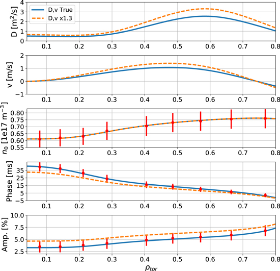
Figure 6. Synthetic D and v profiles and the resulting steady-state, phase, and amplitude profiles. Dashed orange lines: Blue D and v (called D, v True) profiles multiplied by a factor of 1.3. Example experimental data points and error bars in red to display what kind of features we are able to measure with our CXRS systems. A change resulting from a smaller factor than 1.3 in the transport coefficients cannot be distinguished outside the error bars with the CXRS diagnostic.
Download figure:
Standard image High-resolution imageThe second task was to investigate how a potential MHD mode could affect the profiles. Such a mode could, for example, enhance the transport locally and, thus, give rise to a sharp localized peak in the D profile. The resultant steady-state density, phase and amplitude profiles from such hypothetical D profiles (keeping the v profile constant) are shown in figure 7. The blue lines corresponds to the same profiles shown in figure 6. For the dashed magenta lines, a sharp Gaussian peak in D has been added around ρtor ∼ 0.33, to simulate a 3/2 neoclassical tearing mode [37]. This sharp rise in the D profile leads to a flattening of the steady-state profile n0 at ρtor ∼ 0.33 as well as in the phase and the amplitude profiles. This flattening is still within the experimental error bars for the steady-state and the amplitude, but on the borderline for the phase. It is also interesting to investigate how the sharpness of such a peak affects the profiles. The result of such an investigation is displayed in figure 8. The blue lines are, again, the original profiles and the width of the added Gaussian peak has consequently been increased for the dashed green, magenta, and orange lines. One can see that increasing the width also leads to a flattening of the steady-state, phase, and amplitude profiles. Here, the green case is well within the experimental error bars, the magenta case is borderline for the steady-state and phase, but the orange case is outside the error bars for the steady-state and phase. It is obvious to see that such a small feature in the dashed green steady-state profile can probably not be distinguished from the blue case within the error bars, whereas it should not be a problem to distinguish between the orange and the blue cases. However, given the width of the peak in the magenta and orange case, the peak cannot be classified as localized anymore. The fact that a very large change in the D or v profile only leads to small changes in the experimental data, that is in the steady-state, phase, and amplitude, stems from the ill-posedness of the inverse problem. This further strengthens the argument that when solving such an inverse problems, some kind of regularization must be applied in order to heal the ill-posedness. To conclude, it would be difficult to distinguish a mode outside of the error bars with our CXRS systems, since such a mode has to cause a peak with a very high diffusion and/or be very broad, in which case the mode would not be localized anymore.
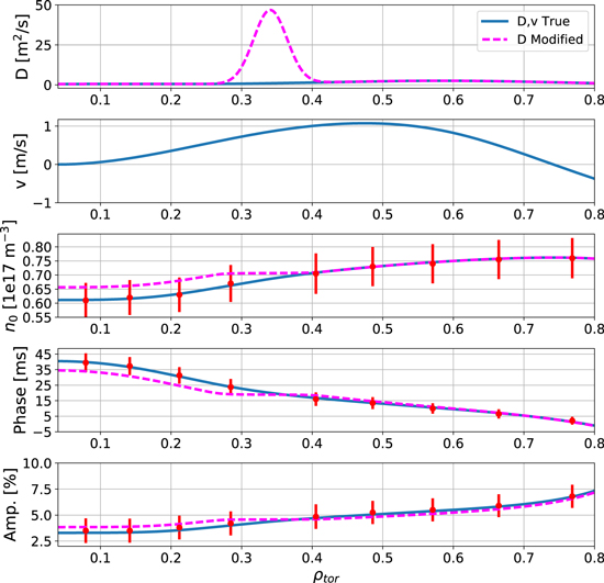
Figure 7. Synthetic D and v profiles and the resulting steady-state, phase, and amplitude profiles. To simulate a MHD mode, a peak in the D profile has been added (dashed magenta lines) on top of the original profile (blue lines). The v profile was kept constant. Example experimental data points and error bars in red to display what kind of features we are able to measure with our CXRS systems.
Download figure:
Standard image High-resolution image
Figure 8. Synthetic D and v profiles and the resulting steady-state, phase, and amplitude profiles. To simulate a MHD mode, peaks in the D profile with different widths have been added (dashed green, magenta, and orange lines) on top of the original profile (blue case). The v profile was kept constant. Example experimental data points and error bars in red to display what kind of features we are able to measure with our CXRS systems.
Download figure:
Standard image High-resolution imageAs an additional check, our radial transport solver was benchmarked against the impurity transport code STRAHL [12], which solves the forward problem. The final D and v profiles from our solver were given to STRAHL as inputs to cross-check the simulated steady-state density n0 and the phase and amplitude of the modulation (see section 4 on how the phase and amplitude are calculated). As can be seen in figure 9, there is an excellent agreement in all quantities between the two codes. However, the radial transport solver developed in this work was able to perform one forward calculation in a few milliseconds, whereas STRAHL, which deploys an additional computational expensive time discretization using the Crank–Nicolson scheme, needs several seconds for the same task. In fact, in some cases the complete minimization procedure is finished in the same time it takes STRAHL to complete one forward calculation. The fact that the inverse problem can be solved in few seconds makes it possible to carry out a brute force uncertainty estimation, described in the next section, in a couple of hours. For such analysis STRAHL would require several days.
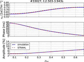
Figure 9. Result of the benchmark of our radial transport solver (blue) with the impurity transport code STRAHL (red). There is a very good agreement in all quantities between the two codes.
Download figure:
Standard image High-resolution image3.2. Uncertainties
As mentioned in section 2.1, the calculation of the experimental boron density via equation (3) is subjected to several different uncertainties. The first one is the error on the measured CXRS line intensity, which is well known and characterized. The second one is the uncertainty on the atomic data that goes into the effective charge exchange emission rates  , which is estimated at ∼15%–20%. The changes in
  are dominated by the interaction energy, which is constant in our case. Changes due to the electron density, ion, and electron temperatures along the beams are minimal, and, therefore, this uncertainty does not significantly impact the error on the overall profile shape, which is of interest in our case. The third and final one is the uncertainty in the determination of the neutral beam density. This in turn depends on the uncertainties of the beam stopping rates, the beam geometry as well as the measured electron density. The same argument as above applies to the beam stopping rates, i.e. they do not significantly affect the profile shape error bar and have, therefore, been neglected. The beam geometry is well diagnosed and benchmarked by the two different NBI systems as well as by cross-checking that the same answer is obtained when using different beam combinations. The electron density ne has the biggest impact on the attenuation of the neutral beam. If the standard deviation on the electron density was known, this uncertainty could be added to the overall uncertainty on the neutral beam density. However, the electron density is deduced from an integrated data analysis framework [38], where the measured electron densities from several different diagnostics have been combined into one profile using Bayesian inference and this procedure does not produce a standard deviation, but rather confidence bands on the electron density, which cannot be used in a standard error propagation scheme. Therefore, this last source of error is not routinely included in the overall uncertainty on the impurity density, but can be tested by running the analysis with variations of the electron density.
The measurement data nB(rl, tk) =  is, therefore, subjected to an error such that each data point is normally distributed
  with standard deviation
  . The relative error on the boron density is difficult to assess (see discussion above) and, therefore, the error on the boron intensity
  is used for
  . To assess the uncertainties on the measured transport coefficients, a full Monte Carlo approach is used, where this multi variate normal distribution of the experimental data
  is assumed. NS = 10 000 random samples are drawn from this distribution and every sample goes through the simulation procedure described in section 2.3, thus resulting in a posterior distribution. The posterior distribution itself, however, is not normally distributed even though the samples were drawn from a normal distribution. The reason for this is because the transport equation is nonlinear. The uncertainty bands of the D and v profiles shown in the next section are pointwise confidence intervals of 95% of the posterior distribution. These confidence intervals of the D and v profiles, therefore, only represent a statistical error. Other non-statistical uncertainties most certainly also play a role, but require a full Bayesian framework, which is outside the scope of this work.
4. Experimental results and comparison to theory
The experimental data presented here is from an H-mode plasma with a toroidal magnetic field of 2.5 T at the magnetic axis, a plasma current of 0.8 MA, and an edge safety factor q95 of 5.2. The heating scheme was as follows: 5 MW of constant NBI, 0.5 MW of constant ECRH, and 1 MW modulation of the ICRF heating power as described in section 2.1. Time traces of the heating powers can be seen in figure 10(c). The modulation frequency of the ICRF heating power, and consequently the frequency of the boron modulation, was 8.33 Hz, which can be seen in figure 1. As mentioned in section 2.1, for this technique to be valid the modulation of the background plasma should be kept to a minimum. Consequently the amplitude of the modulation of the electron density ne (<1%), electron temperature Te (<1%), and ion temperature Ti (3%) at the radial location ρtor ∼ 0.1 were examined. Time traces of these signals as well as of the plasma stored energy (WMHD) are shown in figures 10(a), (b), and (d). Note that these <1% and 3% temperature modulations are near the plasma center where the ICRF is deposited and where the perturbation is the largest. The phase and amplitude profiles of the Te (orange) and Ti (blue) modulations are shown in figure 11 and one can see that they are consistent with direct heating by the ICRF as they peak in the center and have a minimum in phase at this location as well. The phase of for Te is not shown as it is within the noise level and, therefore, not meaningful. We define our region of interest to start at ρtor = 0.25, since these quantities are <1% outside of this location. The even smaller perturbation observed in the ne profile is a very good sign that transport is not changing as a result of the applied perturbations.
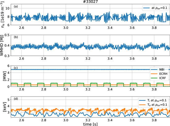
Figure 10. Time traces of the (a) electron density at ρtor = 0.1, (b) plasma stored energy (WMHD), (c) NBI, ECRH, and ICRF heating powers, and (d) electron and ion temperature at ρtor = 0.1 for the dataset presented in this paper.
Download figure:
Standard image High-resolution image
Figure 11. Phase and amplitude of the modulation of Te (orange) and Ti (blue) at the modulation frequency 8.33 Hz. The phase of for Te is not shown as it is within the noise level.
Download figure:
Standard image High-resolution imageThe steady-state boron density profile n0 as well as the phase and amplitude profile of the boron modulation is presented in figure 12. The red points are the mean experimental data points. By fitting the experimental data nB(rl, tk) (left-hand side of figure 3) with the function presented in equation (5), the phase and amplitude profiles can be calculated from the coefficients a(r) and b(r), where the amplitude is given by  and the phase by
  . This will give a phase in units of radians, but it is more intuitive to have the phase in units of seconds, since it represents the propagation time of the modulation. The conversion from radians to seconds can be obtained by dividing the phase, in radians, with 2πf, where f is the frequency of the modulation. The steady-state profile is simply given by n0(r) in equation (5). By performing the same exercise on the reconstructed data shown on the right-hand side of figure 3, these quantities can be extracted and are represented by the blue lines in figure 12. Hence, the blue lines are not fits to the red data points, but rather the results of the minimization. The agreement is very good, which is a sign of the correctness of the method used. One can note several things when studying figure 12. First, in this particular case the steady-state boron density profile is hollow. Second, the phase shift indicates how fast the modulation propagates into the core. In this case the phase shift is ∼35 ms. Third, the amplitude modulation is strongest at the edge where the boron source is located, which also becomes clear by looking at figure 3. In this case, the amplitude of the modulation is ∼7% at ρtor ∼ 0.7.

Figure 12. Steady-state, phase, and amplitude of the measured data (red) and the simulation (blue). The blue lines are not fits to the red data points, but rather the results of the minimization.
Download figure:
Standard image High-resolution imageThe deduced transport coefficients are compared with neoclassical calculations, performed with the code NEO [39, 40], as well as quasi-linear gyrokinetic simulations at a wavenumber kθ = 0.4, computed with the code GKW [41]. Turbulent and neoclassical transport components are summed under the assumption that the turbulent transport heat conductivity matches the anomalous part of the power balance heat conductivity, which is computed with TRANSP [42] (see [43] for more details).
The experimental transport coefficients for the dataset presented in this paper as well as a first comparison to theory are presented in figure 13. Neoclassical diffusion (black squares) is, as expected, much smaller than the measured values (blue curve), and hence, the transport is turbulence driven. In this case, the total theoretical D (magenta points) agrees reasonably well within a factor of 2 with the experimental one, whereas the theoretical v is in the opposite direction. The sign convention of v is the following: a hollow density profile means an outward drift velocity e.g. v > 0. The opposite (v < 0) corresponds to an inward directed drift velocity, which means a peaked density profile. The experimental v profile is positive (outward), which agrees with the hollow steady-state n0 profile in figure 12. Since the theoretical drift velocity is negative, the theory fails to capture this and instead predicts considerably more peaked steady-state profiles than are measured. The fact that the gyrokinetic simulation is unable to fully capture the hollowness of the steady-state profile is consistent with previous experimental studies on carbon transport [44–46] and nitrogen transport [46] at JET and steady-state boron transport at AUG [14, 43, 47], which also observed discrepancies between theory and experiment for hollow impurity density profiles. The uncertainty regions of the D and v profiles in figure 13 are calculated as described in section 3. The end of the gray region indicates where our region of interest starts (ρtor = 0.25).
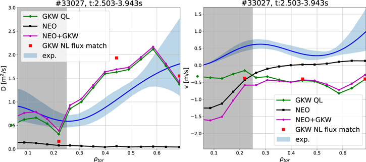
Figure 13. Experimental and theoretical D (left) and v (right) profiles. The experimental profiles with their uncertainty bands are depicted in blue, the ones from the quasi-linear GKW run in green diamonds, from NEO in black squares, and the total theoretical profiles in magenta circles. The red squares represent the result of the nonlinear GKW run performed with matching of the heat fluxes. Our region of interest starts at ρtor = 0.25, hence, where the gray region ends.
Download figure:
Standard image High-resolution imageTo investigate how large an impact the ion temperature modulation has on the transport coefficients calculated by GKW, additional simulations with an averaged maximum and an averaged minimum Ti profile were performed. Maxima and minima of the Ti modulation were chosen and from these profiles an average maximum and minimum Ti profile were created, which were then used as inputs to GKW. The resultant transport coefficients of the new runs (red diamonds and yellow squares) closely follow the original run (blue) except at ρtor ∼ 0.22, which is represented by the error bar in figure 14. The reason for the different results is that the point at this location is highly sensitive to the choice of the spectrum in the calculation of the quasi-linear transport. Different branches are competitively almost equally unstable, but produce very different impurity transport. It can thus be concluded that, overall, the change in the ion temperature gradient due to the small modulation present does not impact the predicted transport coefficients from GKW. As a consistency check, nonlinear GKW runs, both with and without heat flux matching between theory and experiment, at three radial locations were performed. The results of these runs can be seen in figure 15, where D/χi (top) and v/χi (bottom) profiles are plotted. The quasi-linear results are shown in green, the nonlinear without heat flux matching in magenta, and the nonlinear with heat flux matching in red. As can be seen, the nonlinear results agree well with the quasi-linear results, except for the data point at ρtor ∼ 0.22, but this come as no surprise since that point is much more sensitive to the choice of the kθ spectrum (see figure 14 and discussion above) and the nonlinear result includes all unstable modes, while the quasi-linear one is only based on the most unstable [16]. Additionally in figure 15, the experimental profiles are shown in blue. For D/χi, the experimental result is on the order of unity. While in the dimensionless parameters D/χi and v/χi there is a good correspondence between nonlinear and quasi-linear results in figure 15, some differences are particularly visible when the comparison is performed on the dimensional nonlinear with flux matching (red squares) and the reconstructed quasi-linear values (green points) of D in figure 13, as the ion temperature gradients which have been used to match the heat flux had to be modified with respect to the nominal values. This is particularly visible for the D values around mid-radius, for which the logarithmic ion temperature gradient had to be decreased by almost 20%, with a consequent increase of the local value of the corresponding heat conductivity. In contrast, for the inner and outer points, the logarithmic ion temperature gradients had to be increased by less than 10% in order to match the anomalous part of the ion heat flux computed with TRANSP.
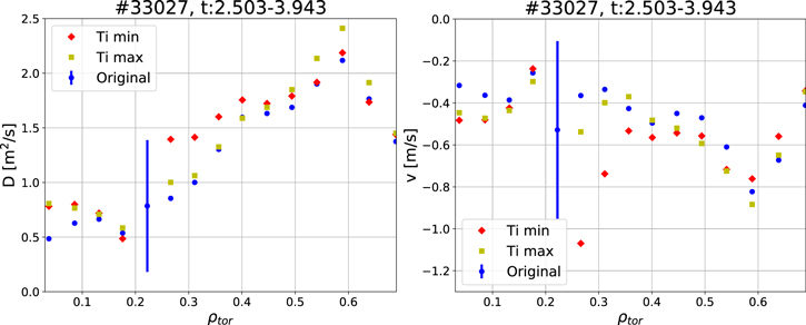
Figure 14. D (left) and v (right) profiles (blue points) from GKW. The error bar at ρtor ∼ 0.22 shows how D and v change in the runs with the average maximum and minimum Ti profile at this particular location. The rest of the data points from these additional runs are shown as red diamonds (Ti minimum) and yellow squares (Ti maximum) and show significantly less variation than at ρtor ∼ 0.22.
Download figure:
Standard image High-resolution image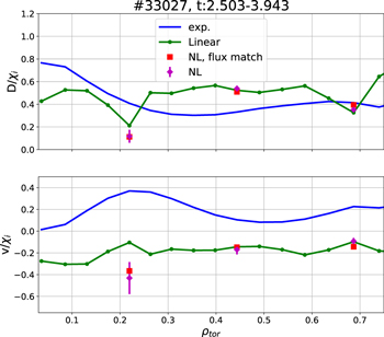
Figure 15. D/χi (top) and v/χi (bottom) profiles from GKW comparing the results from the quasi-linear (green line) with the nonlinear without flux matching (magenta diamonds), and nonlinear with flux matching (red squares) runs. The experimental profiles are shown in blue.
Download figure:
Standard image High-resolution image
5. Conclusion
A new ICRF modulation technique has been developed and exploited at AUG for obtaining time-dependent boron density signals. The technique has been thoroughly tested and applied in several different plasma conditions, one example is shown in this paper. This method requires CXRS data of good quality, i.e. high spatial and temporal resolution. From the CXRS measured boron intensity, the boron density is calculated using effective charge exchange emission rate coefficients and neutral beam densities. With a time-dependent boron density signal at hand, the boron transport coefficients D and v in the radial transport equation are individually determined. This task is done by solving an inverse problem by a quasi-Newton method. The functional form assumed for the boron density is a background steady-state component plus a sum of a cosine and sinus with the frequency of the modulation. Hence, a second requirement is that the boron density signal can be well represented by the sum of a few sinusoidal terms. This implemented framework has been verified with the method of manufactured solutions as well as benchmarked with the transport code STRAHL. The uncertainties of the transport coefficient profiles are estimated with a Monte Carlo procedure, where random samples are drawn from a multi variate normal distribution of the experimental data. The transport coefficients are assumed to be constant in time, which requires a constant plasma background. This implies that the resultant modulation of the electron density, electron temperature, and the ion temperature should be kept as small as possible. It was observed that the modulation of the electron density, temperature, and the ion temperature are less than 1% in the radial region of interest (ρtor > 0.25), whereas the boron density modulation amplitude is 4% in the core and 7% at the edge. The experimental transport coefficients are compared with neoclassical calculations with the code NEO and quasi-linear and nonlinear gyrokinetic simulations with the code GKW. Neoclassical D is well below the experimental D meaning the transport is turbulence driven. The comparison to gyrokinetic theory shows an agreement within a factor of 2 in D, but the theoretical v has the opposite sign, i.e. predicts a more peaked steady-state boron density profile than measured in the experiment. Additional nonlinear GKW runs have been carried out and the nonlinear results agree well with the linear. The analysis, thus, enables us to measure core boron transport coefficients over a wide range of plasmas with error bars on the order of ∼30%. Moreover, this technique and solver are directly applicable in other situations as long as the studied impurity can be measured with high spatial and temporal resolution and there exists a way of modulating the impurity density at the edge in such a way that the resultant density signal is of a sinusoidal-like form. Future work will exploit this method and focus on building up a database of transport coefficients in different plasma conditions, to perform a more comprehensive comparison with the theoretical predictions, and to better characterize the domains of agreement and disagreement.
Acknowledgments
We thankfully acknowledge the financial support from the Helmholtz Association of German Research Centres through the Helmholtz Young Investigators Group program. In addition, this work has been carried out within the framework of the EUROfusion Consortium and has received funding from the Euratom research and training programme 2014–2018 under Grant Agreement No. 633053. The views and opinions expressed herein do not necessarily reflect those of the European Commission.