
Abstract
The ability to compute accurately the strain field in Nb3Sn filaments is a crucial point in cable design, due to the significant strain sensitivity of niobium–tin wires. Due to its heterogeneity, a straightforward numerical simulation of a cable, taking into account all the details of the microstructure, would result in an enormous number of unknowns. As an alternative, multiscale approaches can be used to deal with this kind of problem, to understand the behaviour across the various scales. In this framework, a simple and efficient approach to obtain the homogenized properties of a heterogeneous strand is proposed here. This approach is developed for the non-linear, thermo-mechanical field. It consists of the solutions to some boundary value problems formulated on a suitably chosen statistically representative volume element of the wire. Two bronze-route strands and one internal-tin strand are considered and the equivalent parameters are obtained. Finally, the cool down and the subsequent application of a tensile axial load are simulated taking into account the homogenized wires. Computed results are shown to be in excellent agreement with measured stress–strain curves.
Export citation and abstract BibTeX RIS
1. Introduction
Scientific and medical equipment often require the generation of high magnetic fields, which are obtained by means of superconducting (SC) magnets. Usually, the coil windings of a SC magnet are made of wires or tapes of type II superconductors (e.g. NbTi or Nb3Sn), and the wire or tape itself may be made of tiny filaments (4–20 μm thick) of superconductor in a normal metal (generally bronze or copper) matrix. Nb3Sn cables perform better than NbTi ones, however they are brittle and strain sensitive. Because of its brittleness, the compound Nb3Sn cannot be extruded and drawn (as for example NbTi), but requires special manufacturing processes: a billet including un-compounded precursors of Nb3Sn is assembled and processed until the desired wire size is achieved. After that, wires are twisted to assemble the cable, which is then wound to obtain the coil. Finally, the entire coil is heated up to the reaction temperature (usually 900–950 K) to allow Sn atoms to diffuse and react with Nb atoms to form Nb3Sn precipitates. At the end the coil is cooled down to room temperature and then to its operating conditions (about 4–7 K). During the cool down, a strain field is developed due to the different thermal expansion properties of the wire materials and, when the coil is energized, the wires experience additional strain because of their helix geometry [1, 2] and the Lorentz force acting as a bending load [3–8]. Furthermore, contact phenomena occurring inside the cable cause local peaks of strain components, localized in the strand-to-strand contacts [9–11].
The significant sensitivity of Nb3Sn to strain can be regarded as one of the most important factors responsible for the degradation of cable performances. Therefore the ability to compute accurately the strain field in Nb3Sn filaments is a crucial point in cable design and a considerable effort has been focused on this subject over recent decades [12–19]. However this is not an easy task and it still remains an open issue. Considering the basic items (magnet, cable, wire, filament), they cover several length scales, and each scale plays an important role in the final strain field of Nb3Sn filaments. A straightforward numerical simulation, e.g. via the finite element (FE) method, of the macro-scale magnet taking into account all the details of the lower scales, down to the single filament, would result in an unmanageable number of unknowns. As an alternative, multiscale approaches can be used to deal with this kind of problem, to understand the behaviour across the various scales [20–26]. In this paper a simple and efficient model to bridge the filament level and the wire is presented. The wire is treated on a macro-scale and the Nb3Sn filaments on a micro-scale. The final goal consists of calculating the equivalent characteristics of a wire, to be able to perform our analyses at the macro-scale as if the strand were homogeneous.
2. Material behaviour
Generally Nb3Sn wires are mainly made of three components: copper stabilizer, bronze matrix, and Nb3Sn filaments. Concerning their mechanical behaviour, copper and bronze are elasto-plastic while Nb3Sn is assumed to remain elastic, due to its very high yield limit. It is not easy to find temperature-dependent material properties over the whole temperature range needed (950–4 K). Most of the values used here are taken from [27, 28] and they are summarized in tables 1 and 2.
Table 1. Elastic and thermal characteristics of Nb3Sn, bronze and copper.
| T (K) | E (MPa) | ν | α(1/K) |
|---|---|---|---|
| Nb3Sn | |||
| 923 | 135 000 | 0.3 | 9.535 84 × 10−6 |
| 800 | 135 000 | 0.3 | 9.407 12 × 10−6 |
| 700 | 135 000 | 0.3 | 9.284 04 × 10−6 |
| 600 | 135 000 | 0.3 | 9.144 44 × 10−6 |
| 500 | 135 000 | 0.3 | 8.988 33 × 10−6 |
| 400 | 135 000 | 0.3 | 8.815 68 × 10−6 |
| 293 | 135 000 | 0.3 | 8.612 66 × 10−6 |
| 200 | 135 000 | 0.3 | 8.420 84 × 10−6 |
| 100 | 135 000 | 0.3 | 8.198 63 × 10−6 |
| 4 | 135 000 | 0.3 | 7.969 77 × 10−6 |
| Bronze | |||
| 923 | 90 941 | 0.34 | 2.118 07 × 10−5 |
| 800 | 94 680 | 0.34 | 2.072 44 × 10−5 |
| 700 | 99 210 | 0.34 | 2.047 65 × 10−5 |
| 600 | 104 560 | 0.34 | 2.0278 × 10⁻⁵ |
| 500 | 110 250 | 0.34 | 2.007 26 × 10−5 |
| 400 | 115 800 | 0.34 | 1.980 39 × 10−5 |
| 293 | 121 039 | 0.34 | 1.938 22 × 10−5 |
| 200 | 124 560 | 0.34 | 1.885 05 × 10−5 |
| 100 | 126 810 | 0.34 | 1.805 31 × 10−5 |
| 4 | 127 038 | 0.34 | 1.701 62 × 10−5 |
| Copper | |||
| 923 | 91 711 | 0.376 | 2.118 07 × 10−5 |
| 800 | 96 680 | 0.371 | 2.072 44 × 10−5 |
| 700 | 102 210 | 0.367 | 2.047 65 × 10−5 |
| 600 | 108 560 | 0.363 | 2.0278 × 10⁻⁵ |
| 500 | 115 250 | 0.359 | 2.007 26 × 10−5 |
| 400 | 121 800 | 0.354 | 1.980 39 × 10−5 |
| 293 | 128 109 | 0.350 | 1.938 22 × 10−5 |
| 200 | 132 560 | 0.346 | 1.885 05 × 10−5 |
| 100 | 135 810 | 0.342 | 1.805 31 × 10−5 |
| 4 | 136 998 | 0.338 | 1.701 62 × 10−5 |
Table 2. Yielding (subscript y) and ultimate (subscript u) values of stress and strain for bronze and copper.
| T (K) | σy (MPa) | εy | σu (MPa) | εu |
|---|---|---|---|---|
| Bronze | ||||
| 923 | 26 | 0.0023 | 111 | 0.149 |
| 800 | 51 | 0.0025 | 138 | 0.181 |
| 700 | 70 | 0.0027 | 166 | 0.208 |
| 600 | 86 | 0.0028 | 198 | 0.238 |
| 500 | 103 | 0.0029 | 237 | 0.270 |
| 400 | 120 | 0.0030 | 283 | 0.304 |
| 293 | 141 | 0.0032 | 342 | 0.342 |
| 200 | 165 | 0.0033 | 405 | 0.377 |
| 100 | 204 | 0.0036 | 493 | 0.417 |
| 4 | 343 | 0.0047 | 666 | 0.457 |
| Copper | ||||
| 923 | 13 | 0.0021 | 53 | 0.205 |
| 800 | 15 | 0.0022 | 77 | 0.219 |
| 700 | 18 | 0.0022 | 101 | 0.231 |
| 600 | 23 | 0.0022 | 129 | 0.246 |
| 500 | 30 | 0.0023 | 162 | 0.264 |
| 400 | 38 | 0.0023 | 200 | 0.285 |
| 293 | 49 | 0.0024 | 247 | 0.315 |
| 200 | 59 | 0.0024 | 294 | 0.352 |
| 100 | 72 | 0.0025 | 352 | 0.418 |
| 4 | 86 | 0.0026 | 414 | 0.728 |
The constitutive equations for Nb3Sn, and for bronze and copper in their elastic range, are very simple. They behave like isotropic materials, which means that they have an infinite number of symmetry planes passing through every point. As a consequence, their behaviour depends upon only two constants, i.e. Young's modulus E and Poisson's ratio ν. However, even if the starting material were isotropic, in general the global behaviour of a composite cannot be considered isotropic a priori, since its composite characteristics are determined also by its geometric configuration. Namely, the behaviour of the superconducting wire depends also on the disposition of the filaments inside its matrix.
In general, an elastic constitutive relation can be written as:

where σ is the stress tensor, ε is the strain tensor and D is the (symmetric) fourth-order elasticity tensor. The number of independent components of the elasticity tensor depends on the material's symmetry properties. For fully anisotropic elasticity, i.e. for materials having no symmetry planes, 21 independent elastic stiffness parameters are needed. A class of anisotropic materials are the orthotropic ones, which have two orthogonal symmetry planes and are defined by nine constants. In this case linear elasticity is more easily described by giving the so called 'engineering constants' associated with the material's principal directions 1, 2, 3: the three Young's moduli E1,E2,E3; Poisson's ratios ν12,ν13,ν23,ν21,ν31,ν32; and the shear moduli G12,G13 and G23. These constants define the elastic compliance tensor C (with C = D−1) according to:

where the quantity νij is related to the quantity νji by:
A special subclass of orthotropy is transverse isotropy, which is characterized by a plane of isotropy. In this case, assuming the 1–2 plane (perpendicular to direction 3) to be the plane of isotropy, the following relations hold: E1 = E2 = Ep,ν31 = ν32 = νtp;ν13 = ν23 = νpt,G13 = G23 = Gt; where 'p' and 't' stand for 'in-plane' and 'transverse', respectively. Therefore the stress–strain law contains only five constants and reduces to:
where the quantities νtp and νpt are related to each other by:
and
For the case of deformations caused by a temperature difference ΔT, thermal strains are related to ΔT through the thermal expansion coefficient α of the material. In an isotropic material, a variation of temperature causes only normal strains, equal in all directions, and α corresponds to the strain due to a unitary temperature difference. In a coupled thermo-mechanical problem, the total strain is:

where δij is Kronecker's tensor. In a composite material, the thermal expansion coefficient may assume different values according to the different directions.
Considering the non-linear case, the material behaviour at a point is dependent on its corresponding stress and strain states. For this reason, in non-linear multiscale models, the homogenized (also called 'effective') properties have to be determined point wise at the current stress and strain state.
Given the usual layouts for Nb3Sn, without a lack of generality one can reasonably assume that wires behave in an orthotropic manner. Furthermore, we can expect transverse isotropy in the cross section planes, since filaments are generally embedded in an 'almost axial symmetric' way. However, in keeping with the most general case, in this work we will assume fully anisotropic behaviour, and possible symmetries in the effective material properties will be determined from the numerical results.
3. Computational micro–macro modelling
Superconducting wires are composite materials with a metal matrix and long fibrous inclusions. As already mentioned, a spatial discretization taking into account all heterogeneities would result in a set of equations containing an enormous number of numerical unknowns, thus requiring a computational effort beyond current computer capacities. In addition, even if that set were solved, it would be extremely difficult to handle the amount of data obtained, so that it would be impossible to draw the desired macro-behaviour of the composite. For these reasons, we resort to homogenized material models. Usually the approach is to seek a constitutive law between mean fields, relating volume averaged variables. The volume averaging takes place over a 'representative volume element' (RVE), which is a statistically representative sample of material. Particular attention should be paid to the choice of the RVE: it has to be large enough to contain a sufficient number of heterogeneities, but small enough to be seen as a material point on the macro-scale.
To obtain the volume averages of the desired fields, a series of boundary value problems with test loadings must be solved on the RVE. A commonly accepted micro–macro criterion used in homogenization methods is the Hill condition [29]:

where σ and ε are the stress and strain tensor fields within the RVE of volume |Ω|, and:
Provided that the representative volume element is correctly chosen and for a perfectly bonded heterogeneous body, pure linear displacements of the following form, applied at the boundary of the RVE, surely satisfy Hill's criterion:

where  is a constant strain tensor and x is the position vector.
In this framework, the effective constitutive tensor D* provides a relation between the following averages:

This contains the effective properties of the heterogeneous material and is the elasticity tensor which can be used in the macro-scale analysis. In the same manner, other effective properties, such as the thermal expansion coefficients, can be described, relating the corresponding volumetrically averaged field variables.
The testing procedure to find D* is made up of six independent kinematic loadings of the form (7), each one providing six different averaged stress components and hence six equations for the constitutive parameters present in D*. In this way, a total of 36 relations are generated, which are sufficient to calculate the 36 parameters  of the general, fully anisotropic case and to check the symmetry of the tensor (21 independent constants). It is interesting to note that if the macroscopic behaviour could be considered isotropic a priori, then only one, appropriate, test loading (instead of six) would be sufficient to determine the effective bulk and shear moduli.
In all the considered cases, we have solved the elementary problems via a computational approach using the finite element method and by applying the following kinematic loading conditions:
where λ is a constant parameter.
Once the homogenized elasticity tensor D* (and therefore the compliance tensor C*) is known, in order to calculate the effective thermal expansion coefficients, a unitary temperature difference has been applied to the representative volume element, with zero displacement at the border. Considering the corresponding volume averages of the quantities in equation (4), and assuming, in the general case, an anisotropic thermal behaviour, we obtain:

where vector α collects the homogenized thermal expansion coefficients relative to the different directions.
Once the effective parameters have been obtained, an analysis at the global level can be performed and the total strain components  can be computed. Consequently, the strain field in each different material of the wire can be easily calculated according to equation (4).
4. Representative volume elements and finite element approach
Homogenized properties of the heterogeneous Nb3Sn wires were calculated in the coupled thermo-mechanical field. Temperature-dependent characteristics were considered (tables 1 and 2), so that effective material parameters were calculated for several reference temperatures in the range 4–923 K. To demonstrate the method, three different superconducting wires were taken into consideration. In detail, the strands produced by the companies European Advanced Superconductor (EAS), Furukawa (FUR) and Luvata (LUV) are considered (figure 1). The related RVEs are obtained starting from a scanning electron microscope (SEM) image of the strand. As it is exemplified in figure 2 for the FUR wire, by averaging the radii of filaments and their mutual distances, a statistically representative volume element was obtained. As far as the microstructure is concerned, we can say that RVEs are similar for the FUR and EAS strands, i.e. we can consider a bronze matrix where Nb3Sn filaments are embedded (the distribution of filaments and volume element dimensions are obviously different). On the contrary, the LUV representative volume is made of three initial materials: a bronze matrix (yellow elements in figure 3) where Nb3Sn filaments (light blue elements) are inserted, and a corner of copper (orange elements) .
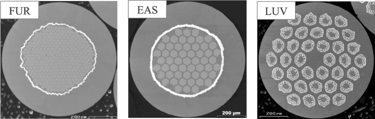
Figure 1. Strands from the companies Furukawa (FUR), European Advanced Superconductors (EAS), and Luvata (LUV). Courtesy of P Lee, University of Wisconsin-Madison Applied Superconductivity Center.
Download figure:
Standard image
Figure 2. Identification of the representative volume element for the wire made by the company Furukawa. SEM image (right) courtesy of P Lee, University of Wisconsin-Madison Applied Superconductivity Center.
Download figure:
Standard image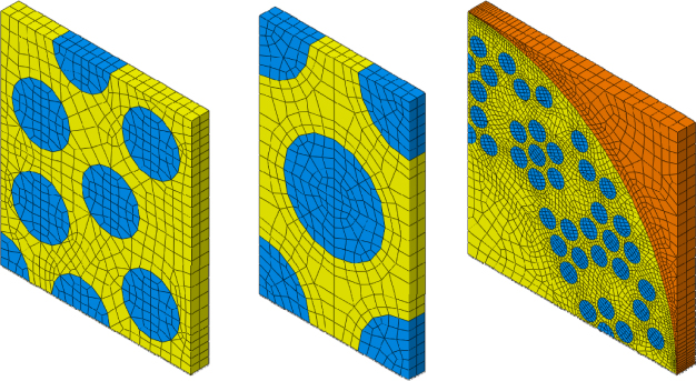
Figure 3. Statistically representative volume elements for the three wires considered: FUR, EAS and LUV from left to right. Yellow elements: bronze matrix; light blue elements: Nb3Sn filaments; orange elements: copper matrix.
Download figure:
Standard imageWe consider three-dimensional problems and refer to a Cartesian coordinate system, with x and y axes defining the plane of the cross section of the wire, and z lying on its axis. By using the finite element method, we solve numerically six mechanical boundary value problems defined by the kinematic loading conditions (7) and (9), compute the effective parameters  and by inversion obtain
  . Finally we solve a thermo-mechanical problem by applying a unit temperature increase to the representative volume and compute the thermal expansion coefficients according to equation (10). This procedure is repeated for ten reference temperatures, for a total of 70 finite element analyses for each wire. In figure 3 the finite element mesh of the statistically representative volume element for the three strands is shown, while a schematic diagram of the boundary value problems considered is drafted in figure 4.
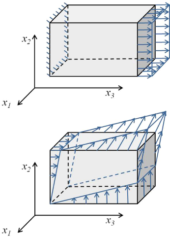
Figure 4. Schematic of the boundary conditions considered for the finite element analyses. The first image illustrates a kinematic load of the first, second and third type from equation (9), the second image illustrates the fourth, fifth and sixth types.
Download figure:
Standard image5. Effective properties
5.1. FUR and EAS wires
FUR and EAS are bronze-route strands, where thousands of filaments are embedded in a bronze matrix. A tantalum barrier separates this inner core from the outer, high purity copper. In the following, the effective properties of the Nb3Sn-bronze area are calculated. The mechanical finite element analyses are non-linear, because they were performed in large displacement and by considering elasto-plastic bronze.
First of all we can say that most  of the coefficients result in zero, so that the strand globally behaves like an orthotropic material. In fact, the effective compliance tensor C* obtained is of the form (3a), and as an exemplifying case, the resulting matrix
  for the FUR wire at room temperature is reported in table 3.
Table 3. Components of the elastic compliance tensor C* calculated for FUR wire at room temperature (1/MPa).
| 7.92 × 10⁻⁶ | −2.59 × 10⁻⁶ | −2.57 × 10⁻⁶ | 0 | 0 | 0 |
| −2.59 × 10⁻⁶ | 7.91 × 10⁻⁶ | −2.57 × 10⁻⁶ | 0 | 0 | 0 |
| −2.57 × 10⁻⁶ | −2.57 × 10⁻⁶ | 7.91 × 10⁻⁶ | 0 | 0 | 0 |
| 0 | 0 | 0 | 2.12 × 10⁻⁵ | 0 | 0 |
| 0 | 0 | 0 | 0 | 2.09 × 10⁻⁵ | 0 |
| 0 | 0 | 0 | 0 | 0 | 2.09 × 10⁻⁵ |
For the chosen ten reference temperatures, the stress–strain curves of the composite material obtained in the directions x,y and z are summarized in figures 5 and 6 for the FUR and EAS strands, respectively. In these plots, the initial slope of the curves identifies the Young's moduli Ei, while the slope of the second part indicates the behaviour during the plastic phase and is usually called the 'plastic modulus'.
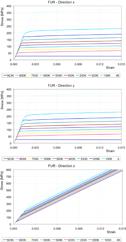
Figure 5. Stress–strain curves obtained for the FUR wire. The behaviour along the x and y directions is almost identical, while along the longitudinal axis z the wire is stiffer in the plastic phase.
Download figure:
Standard image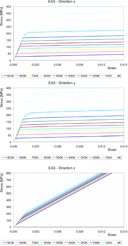
Figure 6. Stress–strain curves obtained for the EAS wire. The behaviour in the cross section is isotropic, and is almost identical to the FUR wire. Along the longitudinal axis z the wire is stiffer in its plastic phase.
Download figure:
Standard imageAs a first remark it can be noticed that, once the bronze matrix is yielding, the deformation is driven by the presence of Nb3Sn filaments, which have a higher elastic modulus and remain elastic. Furthermore, stress–strain curves clearly show that the wire behaviour is transversal isotropic: the results obtained along the x and y directions are almost the same, both in the initial elastic phase and also thereafter. It can also be noticed that in the elastic range also the longitudinal behaviour is very similar to the transversal behaviour. On the contrary, the wires are stiffer along the longitudinal axis in the plastic range, as is testified by the higher slopes of the second part of the curves obtained for the z direction with respect to those obtained for the x and y directions.
To understand the behaviour more clearly during the elastic–plastic regime, as an example the stress–strain curves along the three directions have been collected in one graph, for the FUR wire at room temperature (figure 7). All the other cases, for all wires (FUR, EAS and LUV), are similar. As stated, it can be seen that the behaviour in the cross section of the strand (x–y plane) is isotropic, and in the elastic phase it differs only slightly from the response along the z axis. As soon as the yielding limit is reached, the strand can still be assumed isotropic in the x–y plane (red and blue lines), while longitudinally a higher plastic modulus has to be considered (green line).

Figure 7. Comparison between the behaviour along the x,y and z directions for the FUR wire at room temperature (293 K).
Download figure:
Standard imageFinally, in figure 8 the Young's moduli along the three principal directions are reported as a function of temperature for the FUR and EAS wires: the three resulting elastic moduli along the three directions are almost equal. In a similar way, the shear moduli of the FUR and EAS wires are illustrated in figure 9. Numerical calculations show that in the elastic range, with a little approximation, the effective material can be considered isotropic: Ex = Ey ≈ Ez;Gxz = Gyz ≈ Gxy.
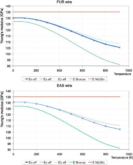
Figure 8. Young's modulus E as a function of temperature for the FUR and EAS wires. The transversally isotropic behaviour is clearly visible for both wires. Furthermore, Young's modulus along the z direction is similar. As a matter of comparison, bronze and Nb3Sn values are also shown.
Download figure:
Standard image
Figure 9. Shear modulus G as a function of temperature for the FUR and EAS wires.
Download figure:
Standard imageFinally, once the mechanical behaviour had been determined, it was possible to calculate the thermal expansion coefficients along the three principal directions for each reference temperature. These are shown in figure 10. It can be seen how they are almost identical along the x,y and z directions, thus revealing an isotropic thermal behaviour: αx = αy ≈ αz.
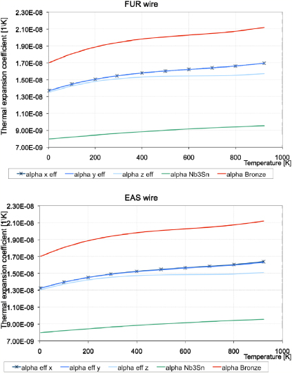
Figure 10. Thermal expansion coefficients obtained for the FUR and EAS wires along the x,y and z directions.
Download figure:
Standard image5.2. LUV wire
LUV wire is of internal-tin type and its microstructure is a little different to those of FUR and EAS. The reacted wire presents islands of Nb3Sn filaments embedded in a bronze area, each one separated from the outside copper by a thin barrier. Also in this case the behaviour in the elastic phase is orthotropic, with there being little difference between the stiffness obtained in the cross section and along direction z. For the ten reference temperatures considered, the stress–strain curves of the composite wire obtained in directions x,y and z are plotted in figure 11. In figure 12 the Young's moduli and shear moduli are reported as a function of temperature. The calculated thermal expansion coefficients are shown in figure 13. The same considerations made for the previous two wires apply also to this strand: the global behaviour is orthotropic in the non-linear phase, while during its linear behaviour the LUV wire can be considered to be approximately isotropic: Ex = Ey ≈ Ez;Gxz = Gyz ≈ Gxy. For its thermal characteristics, again it can easily be seen that αx = αy ≈ αz.

Figure 11. Stress–strain curves obtained for the LUV wire. The behaviour in the cross section is isotropic, while along the longitudinal axis z the wire is stiffer in its plastic phase.
Download figure:
Standard image
Figure 12. Young's modulus E and shear modulus G as a function of temperature calculated for the LUV wire.
Download figure:
Standard image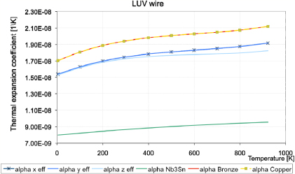
Figure 13. Thermal expansion coefficients along the three directions x,y and z calculated for the LUV wire as a function of temperature.
Download figure:
Standard imageFinally, as a matter of comparison, in figure 14 stress–strain curves along the directions x,y and z are plotted for the three wires at room temperature. In the elastic phase they show the same elastic modulus (initial slope of the curves), but the LUV wire reaches its yielding limit well before the other two.

Figure 14. Comparison of the stress–strain curves obtained along the three directions at room temperature for the FUR, EAS and LUV wires.
Download figure:
Standard image6. Macro-scale analysis and comparison with experimental tests
Once the equivalent homogenized characteristics have been calculated, it is possible to perform the analyses at macro-level. The finite element meshes for the FUR and EAS wires are almost equal. Small differences are due only to the inner and outer radii of the tantalum barrier. In both cases, an inner core of homogenized material can be distinguished, together with a layer of tantalum and an outside ring of high conductivity copper. Concerning the LUV strand, and given its RVE previously chosen, the discretization for the macro-level simulation is made of squares of homogenized material embedded in a copper matrix. The finite element meshes used and the corresponding RVEs are shown in figure 15. Having at hand the results for the experimental tests from [30], the complete cool down from the reaction temperature (923 K) to working conditions (4.2 K) was simulated. It can be assumed that the strand components are in equilibrium at 923 K without stress and strain components; these components are relaxed since the wires remain at high temperature for several hours, and at 923 K the SC compound is formed. After the cool-down step, an axial load was applied to the wire and the load versus displacement path was recorded, from which the average strain versus average stress curve was calculated. This thermo-mechanical simulation was repeated for the three strands. In figure 16 the results for the experimental tests taken from [30] are shown, while in figure 17 numerical results are plotted. Excellent agreement can be seen between results for the experiments and those for numerical simulations. For FUR wire, especially in the first part of the curve, the measured results are slightly below the stress–strain curve obtained from computations. This is probably due to initial alterations in the wire sample, as described in [30].
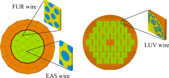
Figure 15. Finite element discretization used for the simulations at macro-level with a snapshot of the related RVEs. Light green elements are of homogenized material, orange elements are of copper and the ring of red elements on the left image is the tantalum barrier.
Download figure:
Standard image
Figure 16. Experimental stress–strain characteristics at 4.2 K for reacted wires taken from [30]. LMI stands for 'LUV', and VAC stands for 'EAS', from the former names of the two manufacturers. SMI is another type of wire, not considered in this work.
Download figure:
Standard image
Figure 17. Results for the simulations at macro-level: calculated average stress versus average strain curves for FUR (violet line), EAS (red line) and LUV (blue line) strands.
Download figure:
Standard image7. Concluding remarks
A simple and effective method has been presented for the numerical homogenization and multiscale analysis of superconducting wires. This method is based on virtual testing of suitably chosen representative volume elements. Provided that the correct boundary conditions are considered, this is founded on a reliable and consistent micro–macro approach. To obtain the homogenized properties, seven boundary condition elementary problems have to be solved at each reference temperature. The introductory work may appear long, however usually the RVE mesh is very simple so that these preliminary computations are very fast. On the other hand once the effective behaviour is determined, the analysis at the macro-level can be performed with a coarse mesh, without taking into consideration all the details at the micro-level. This approach completely defines the three-dimensional behaviour of the composite wires, including transversal contraction and Poisson's effect.
With respect to the author's previous works [20, 21], besides the robustness of the method and its generality, one of the most important points is that no a priori assumptions are needed. The equivalent behaviour results directly from numerical computations. In [20] asymptotic homogenization is illustrated, and in that case the periodicity of the microstructure is necessary in order to apply the method. In [21] three different homogenization approaches are presented and compared, including a numerical procedure very similar to the one explained here. However, in that paper orthotropic behaviour is assumed a priori, while in this work full anisotropic behaviour is considered to remain for the most general case.
In the approach presented, no particular hypotheses are formulated, neither on geometry nor on the material. The most important benefit of this method is that it can be applied regardless of the type of wire on hand.
For the wires studied, starting from a SEM image of the cross sections, the representative volume elements are identified and the effective mechanical and thermal behaviours are calculated. The equivalent parameters obtained show that in the elastic range the composite material can be considered isotropic with a little approximation. In the plastic regime, the material can be considered orthotropic and transversally isotropic. Also the resulting equivalent thermal expansion coefficients are similar along the three principal directions.
This is a significant outcome, because it testifies that at cable level it is possible to consider a relatively simple equivalent behaviour for the wire. The analyses performed constitute an important advantage for future numerical simulations: by using the outlined constitutive law it will be possible to simplify considerably the computations, obtaining a better convergence in the non-linear cases and thus a shorter computational time.
Finally, at the wire level, the calculated results were compared to the available experimental tests. A very good agreement was seen between the computed stress–strain curves and the measured curves. Concerning this point, it is important to underline that the initial properties of the material are unavoidably affected by uncertainty. In the same way, a certain variability is recorded in the measured data, depending upon several factors, e.g. handling of samples, different production billets, difficulties in measurements, etc. Therefore, although the outstanding match recorded between numerical and experimental results is encouraging and useful to illustrate the potential for this method, it cannot be regarded as a definitive validation.
As a further development of this study, a sensitivity analysis of the influence of the material characteristics on the overall stress–strain behaviour of the wire is planned and constitutes the subject of a future paper.
Acknowledgments
Support for this work was partially provided by the Italian National Research Project STPD08JA32_004, 'Algorithms and Architectures for Computational Science and Engineering'. This support is gratefully acknowledged. I would also like to thank Eng. Mattia Pizzocaro from the University of Padova for his valuable contribution on finite element analyses.